Sequence-of-Returns Risk: Why the Order of Your Returns Decides Your Retirement
Key takeaway
The same 30 years of US 60/40 returns that exhausted a 4% withdrawal after 25.2 years from January 1966 would have ended with $1.75 million of every $1 million in reverse order. Across 1,510 retirements since 1871, the order of returns alone accounts for about half of the variation in safe withdrawal rates, and one bad year costs most in the ten years either side of retirement.
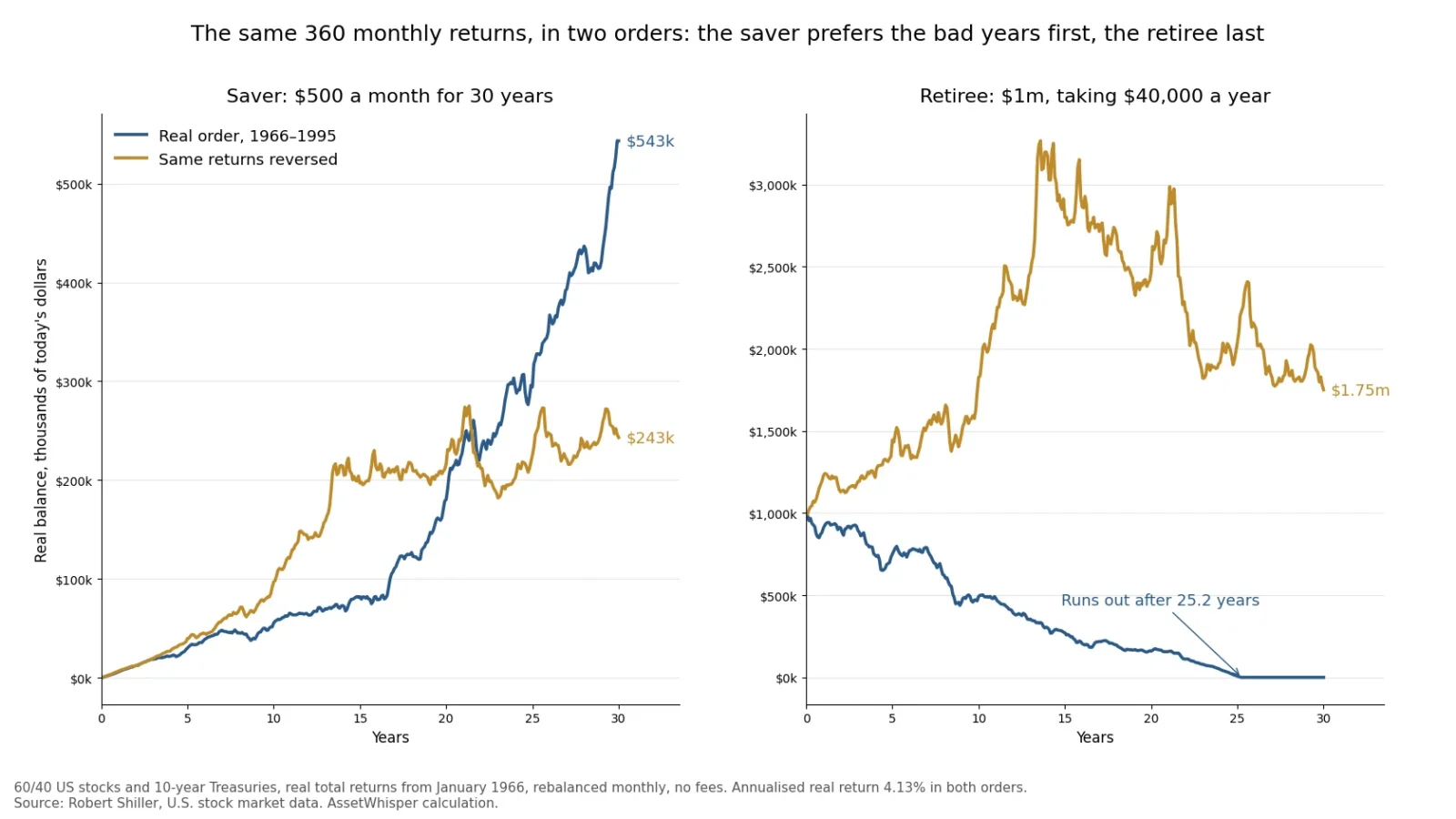
Two retirees can earn exactly the same return over 30 years and end up in opposite places: one with more money than they started with, the other with nothing. The only difference is the order in which the returns arrived. That is sequence-of-returns risk, and it is the reason a retirement plan cannot be judged by its average return.
We measured it on every US retirement that has run its full 30 years since 1871, 1,510 monthly starts, with a 60/40 portfolio and Robert Shiller’s real total-return data to October 2026:
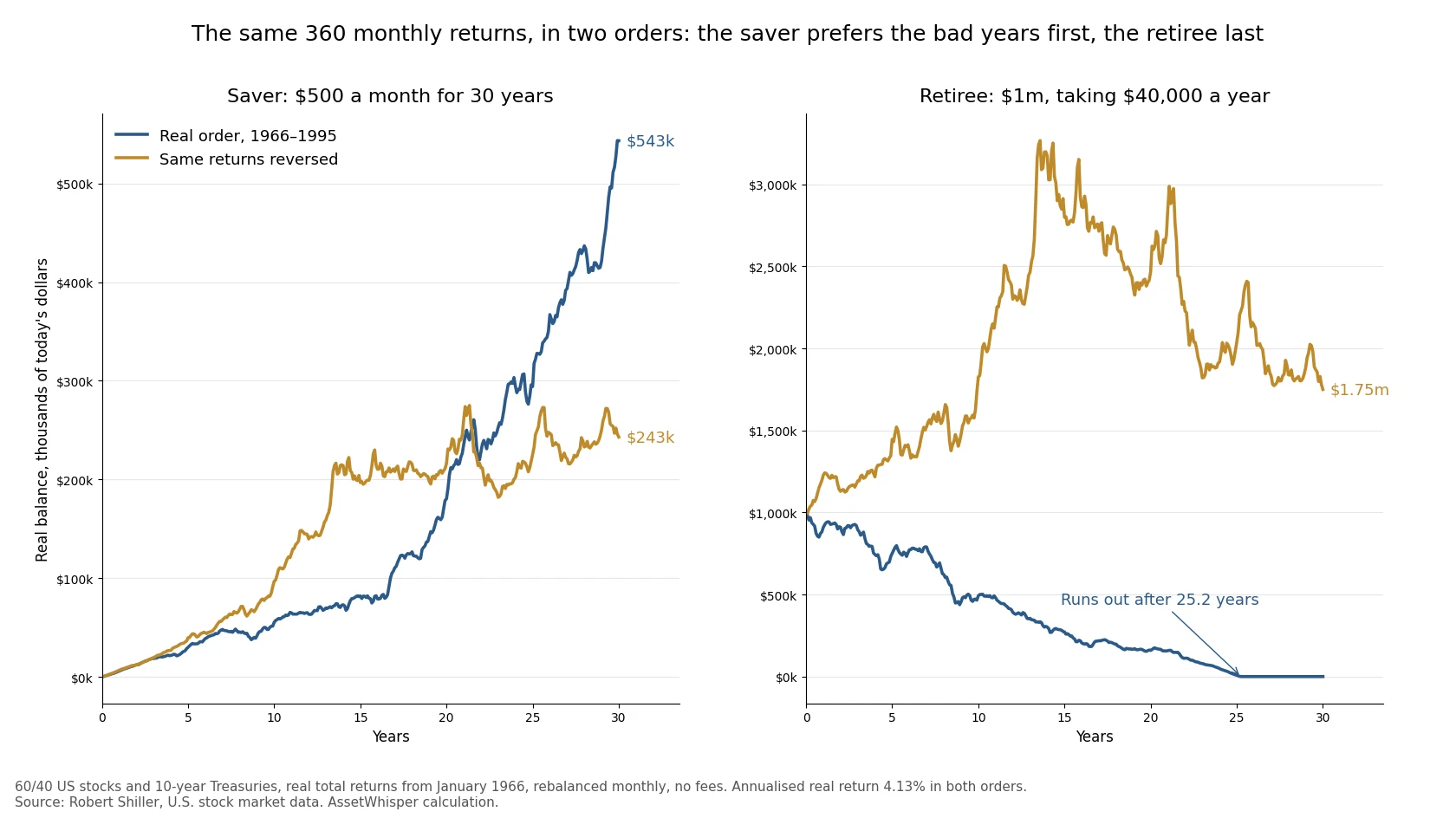
- Order alone can decide the outcome. The returns from January 1966 ran out a $40,000-a-year withdrawal from $1 million after 25.2 years. The same returns in reverse order ended with $1.75 million. The average return was 4.13% a year in both cases.
- About half of the variation in outcomes is order. When we kept each retirement’s own returns and only reshuffled them, the order accounted for 51% of the variation in safe withdrawal rates across all 1,510 starts.
- The danger zone is the decade either side of retirement. A single −25% year costs 24% of lifetime retirement income on average if it lands within ten years of the retirement date, against 3% to 9% if it lands at either end of a working and retired life.
- The usual fixes trade one risk for another. A rising equity glide path did not improve the worst historical case. Spending guardrails stopped every portfolio from running out, but in the 1966 start they cut income to less than a third of its first-year level.
None of this is a forecast. It is a measurement of how the arithmetic of withdrawals works on the one long record we have.
The short answer, in one table
| The 360 monthly real returns of a 60/40 portfolio from January 1966 | Real order (1966–1995) | Same returns, reversed |
|---|---|---|
| Annualised real return over 30 years | 4.13% | 4.13% |
| Real return in the first 10 years | −1.47% a year | +9.48% a year |
| $100,000 invested once, no withdrawals | $337,079 | $337,079 |
| Saver: $500 a month for 30 years ($180,000 in total) | $543,192 | $243,087 |
| Retiree: $1 million, $40,000 a year | Runs out after 25.2 years | Ends with $1,750,206 |
| Retiree’s balance after 10 years | $492,481 | $1,826,490 |
| Highest withdrawal that lasted 30 years | 3.72% a year | 8.32% a year |
All figures are in today’s dollars, after inflation, with monthly rebalancing and no fees or taxes.
Why the order matters only when money moves
The first row of the table is the key to the rest. With no money going in or out, the order of returns makes no difference at all: $100,000 grows to $337,079 either way, because multiplication does not care about order. A lump-sum investor who never adds or withdraws has no sequence risk.
The moment money moves, it does. Each return applies only to the balance that is invested at the time, so a return matters in proportion to how much money it lands on.
- A saver has the least money at the start and the most at the end. Bad years early land on a small balance and let the saver buy cheaply; bad years late land on almost everything. The saver did better with the real 1966 order, weak first decade and all, because it put the strong years at the end: $543,192 against $243,087.
- A retiree has the most money at the start, and every withdrawal shrinks it. Bad years early land on the largest balance and are made worse by the withdrawals taken while prices are down, which sells assets at low prices and leaves less to recover with. The same 1966 order that suited the saver ran the retiree out of money.
This is the same arithmetic that makes average returns misleading in the first place, which we covered in volatility drag. Withdrawals add a second layer: the timing of the losses, not only their size, sets what is left.
The two extremes show how wide the range is. Taking the 1966 returns and sorting them from best to worst, a retiree could have withdrawn 39% of the starting balance every year for 30 years. Sorted from worst to best, 0.33%. No history will ever be that tidy, but the range says how much of the result the order can carry.
How much of a retirement’s outcome is order
One reversed example proves the mechanism. It does not say how much it matters in practice. For that we kept each of the 1,510 retirements’ own 360 monthly returns and put them in 1,000 random orders, then computed the highest fixed real withdrawal that would have lasted 30 years for each order.
The result: across all starts, the order of returns accounted for 51% of the variation in safe withdrawal rates. Which returns a retiree got, the other half. For a typical start, the range between the 5th and 95th percentile orders of the same returns was 2.8 percentage points of withdrawal, the difference between, say, 4.5% and 7.3% a year.
The 1966 retiree was not unlucky in the returns they got, only in their order. Shuffled, the same returns supported a median withdrawal of 5.65% a year, and 4% lasted in 99.4% of the orders. The real order was worse than 99.7% of them. The same was true of all 48 starts, from April 1964 to January 1969, in which 4% ran out: in random orders of their own returns, 4% lasted 99.1% of the time.
The reverse case is just as instructive. The 91 starts with the lowest 30-year returns, all below 3% a year after inflation, came mostly from 1888–1892 and 1951–1955. Every one of them survived a 4% withdrawal in its real order. Their median first decade returned +6.42% a year after inflation and their median last decade −1.59%: the bad years came when there was less money left to lose. In random orders, 4% would have failed in about one in ten.
The same pattern shows up in a simpler test. The return over the whole 30 years explains 40% of the variation in safe withdrawal rates. The first years explain more, and more with each year added:
| Real return measured over | Share of the variation in the safe withdrawal rate explained (R²) |
|---|---|
| First year of retirement | 15% |
| First 3 years | 36% |
| First 5 years | 54% |
| First 10 years | 75% |
| All 30 years | 40% |
60/40 portfolio, 1,510 monthly starts from January 1871 to October 1996, one-variable regressions. Our calculation from Shiller data.
When a bad year hurts most
The historical record mixes many effects at once. To isolate timing, we built the simplest possible life: 30 years of equal real contributions, then 30 years of equal real withdrawals, with every year earning 5% after inflation except one, which loses 25%. That is roughly the record of a 60/40 portfolio: 5.45% a year after inflation since 1871, and a worst calendar year of −28.2% (1917), followed by −24.6% (1974), −21.1% (1937) and −20.0% (2022). Then we moved the bad year through all 60 years and measured how much retirement income it cost.
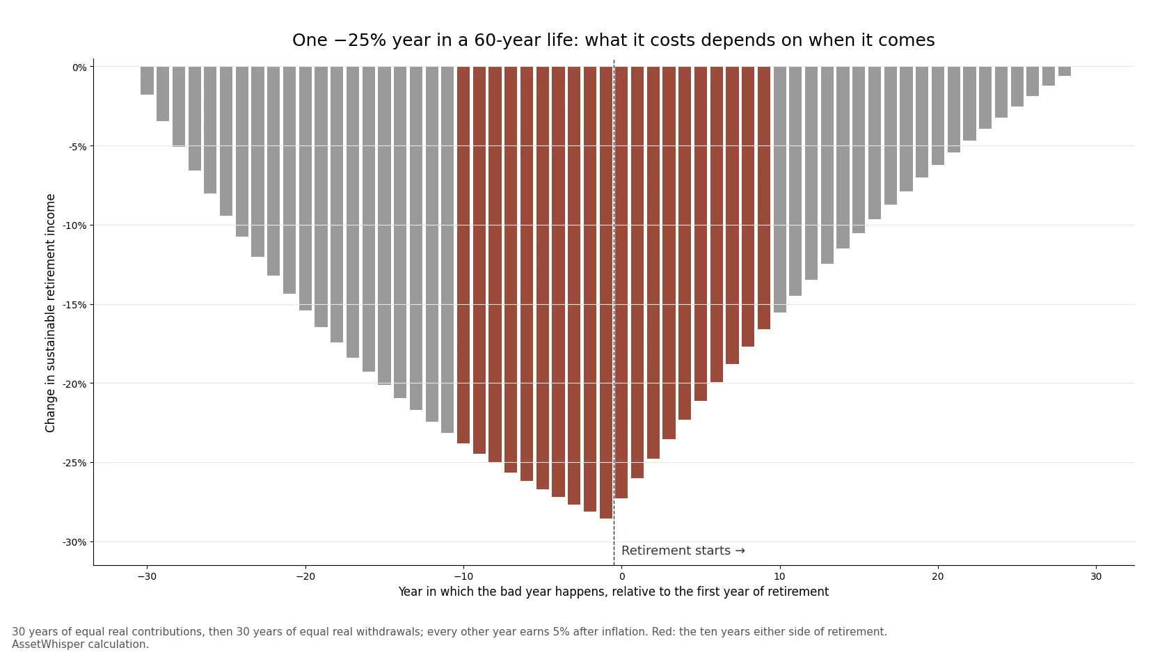
| When the −25% year happens | Change in sustainable retirement income |
|---|---|
| First year of saving (30 years before retirement) | −1.8% |
| 20 years before retirement | −15.4% |
| 10 years before retirement | −23.8% |
| Last year before retirement | −28.6% |
| First year of retirement | −27.3% |
| 10 years into retirement | −15.5% |
| 20 years into retirement | −6.2% |
| Last year of retirement | 0.0% |
The cost peaks in the year just before retirement, when the balance is at its largest, and falls away on both sides, faster after retirement than before. Averaged over the ten years either side of the retirement date, one bad year cost 24.1% of retirement income. In the first ten years of saving it cost 8.5%, and in the last ten years of retirement 3.0%.
Two practical points follow. First, sequence risk does not start on the day of retirement: the last years of saving are as exposed as the first years of spending, because the money is the same money. Second, the risk fades with time in both directions, which is the arithmetic behind portfolios that hold the least risk around the retirement date. For a retiree who starts with a lump sum and no saving phase, the same bad year lowers the sustainable withdrawal from 6.20% to 4.51% if it comes in year one, to 5.17% in year ten, and to 5.76% in year twenty.
What a bad start looks like in the record
A weak first five years did not doom a retirement in history, but it removed most of the margin:
| Real return of 60/40 in the first 5 years | Starts | Median safe withdrawal rate | Worst | Share where 4% lasted 30 years |
|---|---|---|---|---|
| Below −2% a year | 144 | 4.89% | 3.73% | 93.8% |
| −2% to 0% | 84 | 4.82% | 3.72% | 82.1% |
| 0% to 3% | 236 | 4.86% | 3.83% | 89.8% |
| 3% to 6% | 301 | 5.76% | 4.10% | 100% |
| Above 6% | 745 | 7.69% | 4.50% | 100% |
60/40 portfolio, monthly starts from January 1871 to October 1996. Our calculation from Shiller data.
Every failure of the 4% rule came from a start whose first five years returned less than 3% a year after inflation. The worst cases were not the sharpest crashes but the flat, inflationary stretches: the first decade of the 1966 start lost 1.77% a year in stocks and 1.52% a year in bonds after inflation, so there was nowhere to take the withdrawals from without selling at a loss. Our analysis of the 4% rule covers why the 1960s, and not 1929, set the floor.
A depleted balance is a warning, not a verdict. Of the 102 starts whose real balance had halved after ten years of 4% withdrawals, 69.6% still lasted the full 30 years. Of the 260 whose balance was below 70% of the start after ten years, 81.5% lasted. That is why the point at which to review spending is during the first decade, not after it.
Two ways to reduce it, tested
The obvious defence is a lower withdrawal rate: 3.5% lasted in every start of the record for a 60/40 portfolio. That works, at the cost of spending less in the 97% of histories where 4% would have been fine. Two other ideas are widely recommended, and both can be tested on the same 1,510 starts.
A rising equity glide path
Kitces and Pfau (2014) argued that a retiree should start with a low share in stocks and raise it over time, the reverse of the usual advice. The logic follows directly from the red zone: hold the least in stocks when the balance is largest and most exposed, and more once the danger has passed. To test it fairly, we compared paths with the same average equity share, so that any difference comes from timing and not from holding more or less in stocks overall.
| Equity share over 30 years, 4% fixed real withdrawal | Share where 4% lasted | Worst safe rate | Median safe rate | Share where 5% lasted |
|---|---|---|---|---|
| Rising, 30% → 70% (average 50%) | 95.0% | 3.63% | 5.67% | 61.8% |
| Static 50/50 | 96.4% | 3.67% | 6.02% | 69.3% |
| Falling, 70% → 30% (average 50%) | 96.2% | 3.67% | 6.25% | 74.2% |
| Rising, 30% → 60% (average 45%) | 94.3% | 3.61% | 5.52% | 59.5% |
| Static 45/55 | 95.6% | 3.64% | 5.79% | 64.5% |
| Static 60/40, for reference | 96.8% | 3.72% | 6.33% | 75.8% |
Monthly starts from January 1871 to October 1996, equity share changing in equal monthly steps, rebalanced monthly. Our calculation from Shiller data.
On the US record, the rising path did not help. Its worst case was slightly lower than the static portfolio with the same average, and it gave the higher safe rate in only 17.6% to 17.8% of starts. The reason is in the 1966 start itself: in its first decade bonds lost almost as much as stocks after inflation, so holding more bonds early did not protect anything. A rising glide path is insurance against an early crash in stocks. It is not insurance against an early decade of inflation, and in the US that has been the binding case. The idea may work better in histories where bonds did protect, or under assumptions of lower future stock returns, which is the setting in which it was proposed. On the record available, a static 60/40 beat every path tested here.
Spending guardrails
Guyton and Klinger (2006) proposed rules that adjust spending to the portfolio: cut it when the withdrawal rate rises well above where it started, raise it when the portfolio has grown. We tested a simplified, strict version on a static 60/40: each January, if the withdrawal rate is more than 20% above the initial rate, spending is cut by 10%; if it is more than 20% below, spending rises by 10%. Otherwise it stays fixed in real terms. The original rules also skip inflation adjustments after losing years and stop cutting in the last 15 years; we left those out.
| 60/40, 1,510 starts | Fixed 4% | Fixed 5% | Guardrails from 4% | Guardrails from 5% |
|---|---|---|---|---|
| Money lasted 30 years | 96.8% | 75.8% | 100% | 100% |
| Median of each start’s average income, % of the starting balance | 4.00% | 5.00% | 4.59% | 5.02% |
| Starts with at least one year of income below the first year’s | — | — | 60.2% | 69.0% |
| Lowest year’s income in the worst start, as a share of the first year’s | 0% (ran out) | 0% (ran out) | 39% | 31% |
| January 1966 start: average income over 30 years | 3.36% | — | 2.61% | 2.87% |
| Median balance after 30 years, multiple of the start | 1.31× | 0.71× | 1.41× | 1.00× |
Real terms, no fees or taxes. Our calculation from Shiller data.
The guardrails did what they promise: no portfolio ran out, and starting at 5% they paid a median 5.02% a year, a quarter more than the fixed 4% rule. But the risk did not disappear. It moved from the balance to the income. In 69% of starts the retiree had at least one year of spending below the first year’s, and in the worst starts the cuts compounded: ten-percent cuts in consecutive years left income at 31% of where it began. The 1966 retiree on guardrails from 5% averaged 2.87% of the starting balance a year over 30 years, less than the 3.36% average of the fixed 4% retiree whose money ran out after 25 years. Guardrails are a choice about who absorbs a bad sequence: the portfolio, or the household budget. They work best for retirees with a large share of spending they can actually cut.
What this does not say
- It is one country’s history. The US had one of the best markets of the past 150 years. The 1,510 overlapping starts contain only about five independent 30-year periods, so the shares above are descriptions of the past, not probabilities.
- The shuffle test breaks some real structure. Random orders remove the tendency of markets to follow bad stretches with better ones and of inflation to persist. It measures what order alone can do, not how likely each order is.
- The life-cycle model is deliberately simple. Equal contributions and a constant return outside the bad year isolate timing; real careers and markets are messier, and the exact percentages depend on the 5% and −25% assumptions. The shape does not.
- It ignores fees, taxes and behaviour. A 1% annual fee lowers every withdrawal figure above, and a retiree who sells in a panic during a bad first decade makes the sequence worse, which the behaviour-gap research shows is common.
- It is not a forecast for 2026. Starting valuations have been a strong guide to the first decade, and US stocks start from a CAPE near 40. What that implies, and the TIPS ladder that now removes sequence risk from part of the spending, is in our 4% rule analysis and in the equity risk premium at today’s real yields.
Frequently asked questions
What is sequence-of-returns risk?
It is the risk that poor returns arrive at the wrong time, when the most money is exposed and withdrawals are being taken. The same 30 years of US 60/40 returns from January 1966 exhausted a 4% withdrawal after 25.2 years in their real order, and ended with 1.75 times the starting balance in reverse order, with the same 4.13% average real return.
Does sequence of returns matter if I am not withdrawing?
Not for a single lump sum: with no money going in or out, $100,000 invested in the 1966–1995 returns ended at $337,079 in either order. It matters for a saver, in the opposite direction: someone investing $500 a month did better with the bad years first, $543,192 against $243,087.
How much of retirement success is down to the order of returns?
In our test of 1,510 US retirements since 1871, about half. Reshuffling each retirement’s own monthly returns, the order alone accounted for 51% of the variation in safe withdrawal rates. The return of the first ten years explains 75% of the variation, against 40% for the 30-year average.
When is sequence risk highest?
In the years just before and just after retirement, when the balance is largest. In a simple 60-year model, one −25% year cost an average of 24.1% of retirement income if it happened within ten years of the retirement date, 8.5% in the first ten years of saving and 3.0% in the last ten years of retirement. The peak, 28.6%, was the last year before retirement.
Does a bond tent or rising equity glide path reduce sequence risk?
Not on the US record since 1871. A path rising from 30% to 70% in stocks lasted at 4% in 95.0% of starts with a worst safe rate of 3.63%, against 96.4% and 3.67% for a static 50/50 with the same average equity share. In the worst case, 1966, bonds lost almost as much as stocks after inflation in the first decade, so more bonds early did not help.
Do spending guardrails solve sequence risk?
They stop the portfolio running out, at the cost of income. A simplified Guyton–Klinger rule starting at 5% lasted in every start since 1871 and paid a median 5.02% a year, but 69% of retirees had at least one year of spending below the first, and in the worst start income fell to 31% of its initial level.
How we calculated this
- Data: Robert Shiller’s monthly real total-return series for the S&P Composite and for 10-year Treasuries, January 1871 to October 2026 (release downloaded on 11 November 2026).
- Portfolio: 60% stocks and 40% bonds rebalanced monthly unless stated, in real terms, with no fees or taxes.
- Retirements: 1,510 starts, one per month from January 1871 to October 1996, each lasting 360 months. The withdrawal is fixed in real terms at a share of the starting balance and taken at the start of each month. The safe withdrawal rate of a start is the highest such rate that exhausts the balance exactly at the end of month 360; with withdrawals at the start of each month it has a closed form, the inverse of the sum of the discount factors implied by the path.
- Shuffles: for each start, the same 360 monthly returns in 1,000 random orders (fixed random seed). The order share is the average variance of the safe rate within each start’s shuffles divided by the total.
- Life-cycle model: annual steps, one unit contributed at the start of each of 30 years, then the constant real withdrawal at the start of each of 30 years that the same path can sustain; 5% real return in every year except one at −25%.
- Glide paths change the equity share in equal monthly steps over 360 months. Guardrails are checked each January from the second year, on the withdrawal rate of that year’s spending against the current balance.
- The count is one more than in our 4% rule article because Shiller’s series now runs a month further. The calculation script and its output, kept with the article, reproduce every figure.
Sources
- Robert J. Shiller, Stock Market Data Used in Irrational Exuberance (monthly S&P Composite, dividends, CPI and real total returns of stocks and 10-year Treasuries), to October 2026.
- William P. Bengen, “Determining Withdrawal Rates Using Historical Data”, Journal of Financial Planning, October 1994.
- Michael E. Kitces and Wade D. Pfau, “Reducing Retirement Risk with a Rising Equity Glide Path”, Journal of Financial Planning, January 2014.
- Jonathan T. Guyton and William J. Klinger, “Decision Rules and Maximum Initial Withdrawal Rates”, Journal of Financial Planning, March 2006.
Related reading
- The 4% rule at CAPE 40 — 1,509 retirements since 1871, the 1960s failures and the TIPS ladder alternative.
- Volatility drag — why the average return overstates what a portfolio compounds to.
- Bear markets since 1950 — how deep the falls were and how long the recoveries took.
- Lump sum vs dollar-cost averaging — the saver’s side of the same arithmetic.
- How to manage investment risk — the full hierarchy, from position size to drawdown.
This article is general information, not personalised investment advice. It does not take into account the financial situation, objectives or risk tolerance of any individual reader, and the same text is distributed to all readers. The withdrawal rules and glide paths tested are illustrations, not recommendations. Past performance, real or simulated, does not indicate future results, and capital is at risk.