Volatility Drag: Why the S&P 500’s 11.85% Average Return Compounded at 10.02%
Key takeaway
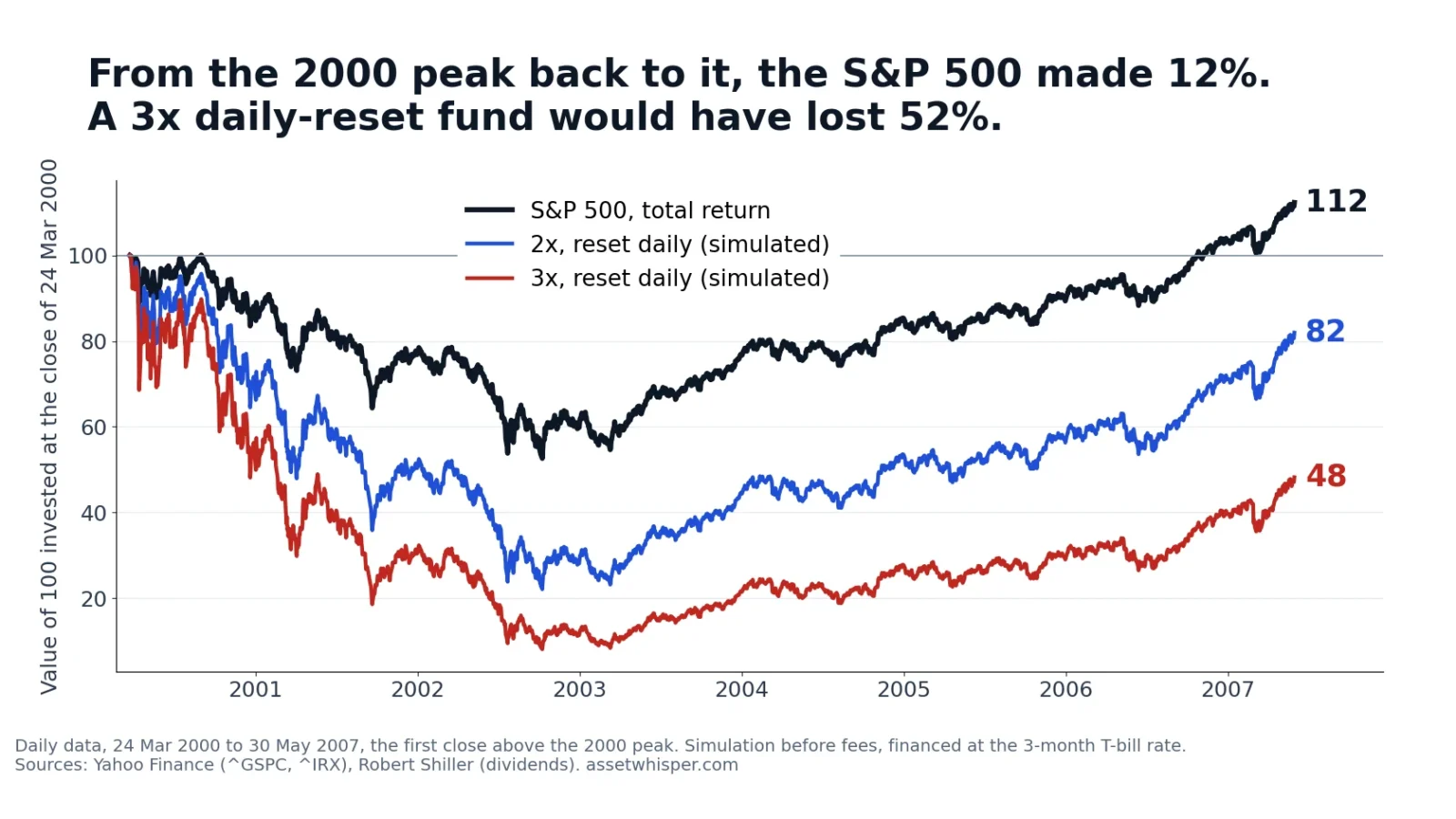
From 1928 to 2025 the S&P 500 averaged 11.85% a year but compounded at 10.02%. The gap, roughly half the variance of returns, is volatility drag. It is why about two in three simulated 30-year histories fall short of an average-return projection, and why a simulated 3x daily fund lost 52% from 2000 to 2007 while the index gained 12%.
Between 1928 and 2025 the S&P 500’s calendar-year returns, dividends included, averaged 11.85%. Money left in the index grew at 10.02% a year. Both figures come from the same 98 yearly returns, and neither is a mistake. The first is the arithmetic mean: add up the yearly returns and divide by 98. The second is the compound, or geometric, rate: the single constant return that turns the starting sum into the final one. The 1.84-point gap between them is called volatility drag, and it is almost exactly half the variance of those yearly returns (1.88 points).
Most explanations stop at “the average return is misleading”. It is not. The arithmetic mean is the right number for the expected value, the average across every history that could have happened. The compound rate is the right number for the typical outcome, what one investor living one history should expect to end with. Volatility drag is the distance between the two, and it grows with volatility, with time and, fastest of all, with leverage. From the March 2000 peak to the day the S&P 500 closed above it again in May 2007, the index returned 12% with dividends. A simulated fund resetting to three times the index every day lost 52%.
The short answer, in one table
Calendar-year returns from Aswath Damodaran’s dataset (NYU Stern), 1928–2025 unless stated. Volatility is the standard deviation of the yearly returns; “half the variance” is the rule-of-thumb estimate of the drag.
| Yearly returns | Average | Compound | Gap | Volatility | ½ variance |
|---|---|---|---|---|---|
| S&P 500, 1928–2025 | 11.85% | 10.02% | 1.84 | 19.40% | 1.88 |
| S&P 500, 1950–2025 | 12.99% | 11.62% | 1.37 | 16.99% | 1.44 |
| S&P 500, 2000–2025 | 9.57% | 7.99% | 1.58 | 17.79% | 1.58 |
| 10-year Treasury bond | 4.82% | 4.53% | 0.29 | 7.90% | 0.31 |
| 3-month Treasury bill | 3.41% | 3.37% | 0.04 | 3.04% | 0.05 |
| 60/40, rebalanced every January | 9.04% | 8.34% | 0.70 | 12.12% | 0.73 |
| US small caps (bottom size decile) | 17.78% | 11.98% | 5.79 | 37.95% | 7.20 |
“Average” is the arithmetic mean of the yearly returns and “compound” the rate money actually grew at. Gaps are in percentage points, computed before rounding. The pattern is the whole story: the gap follows volatility, not return. Treasury bills lose almost nothing between the two averages; the S&P 500 loses close to two points a year; the smallest stocks lose almost six. Ranked by average return, the bottom size decile of US stocks beat the S&P 500 by 5.9 points a year. Ranked by what money invested in them actually did, the lead was 2.0 points.
In money: $100 put into the S&P 500 at the start of 1928 was worth $1,157,009 at the end of 2025. Compounding the 11.85% average for the same 98 years gives $5,862,686, five times what any investor actually received.
+50%, then −50%: why gains and losses do not cancel
Two years are enough to see the mechanism. A gain of 50% followed by a loss of 50% averages zero, but $100 becomes $150 and then $75. The compound rate over the two years is −13.4% a year. A loss always needs a larger gain to undo it, which is why a 50% fall needs a 100% rise to recover, the arithmetic behind every bear market recovery.
| Two years | Average return | $100 becomes | Compound rate |
|---|---|---|---|
| +10%, then −10% | 0% | $99.00 | −0.50% |
| +20%, then −20% | 0% | $96.00 | −2.02% |
| +50%, then −50% | 0% | $75.00 | −13.40% |
| +100%, then −50% | +25% | $100.00 | 0.00% |
The cost scales with the square of the swing. Swings of 10% cost half a point a year; swings twice that size cost four times as much, and swings of 50% cost about 27 times as much. That is where the rule of thumb comes from: compound rate ≈ average return − half the variance, with the variance being the volatility squared. Small swings are almost free. Large ones are not.
Same average, different results
Hold the average return fixed at 8% and change only the volatility. The expected (mean) value of $10,000 after 30 years is the same in every row, $100,627. The typical (median) value is not. “Median, 30 years” is what $10,000 becomes in the middle outcome.
| Volatility | Compound | Drag | ½ variance | Median, 30 years |
|---|---|---|---|---|
| 0% | 8.00% | 0.00 | 0.00 | $100,627 |
| 5% | 7.88% | 0.12 | 0.13 | $97,446 |
| 10% | 7.54% | 0.46 | 0.50 | $88,532 |
| 15% | 6.97% | 1.03 | 1.12 | $75,552 |
| 20% | 6.19% | 1.81 | 2.00 | $60,681 |
| 25% | 5.22% | 2.78 | 3.12 | $45,991 |
| 30% | 4.06% | 3.94 | 4.50 | $32,999 |
| 40% | 1.28% | 6.72 | 8.00 | $14,632 |
| 60% | −5.59% | 13.59 | 18.00 | $1,780 |
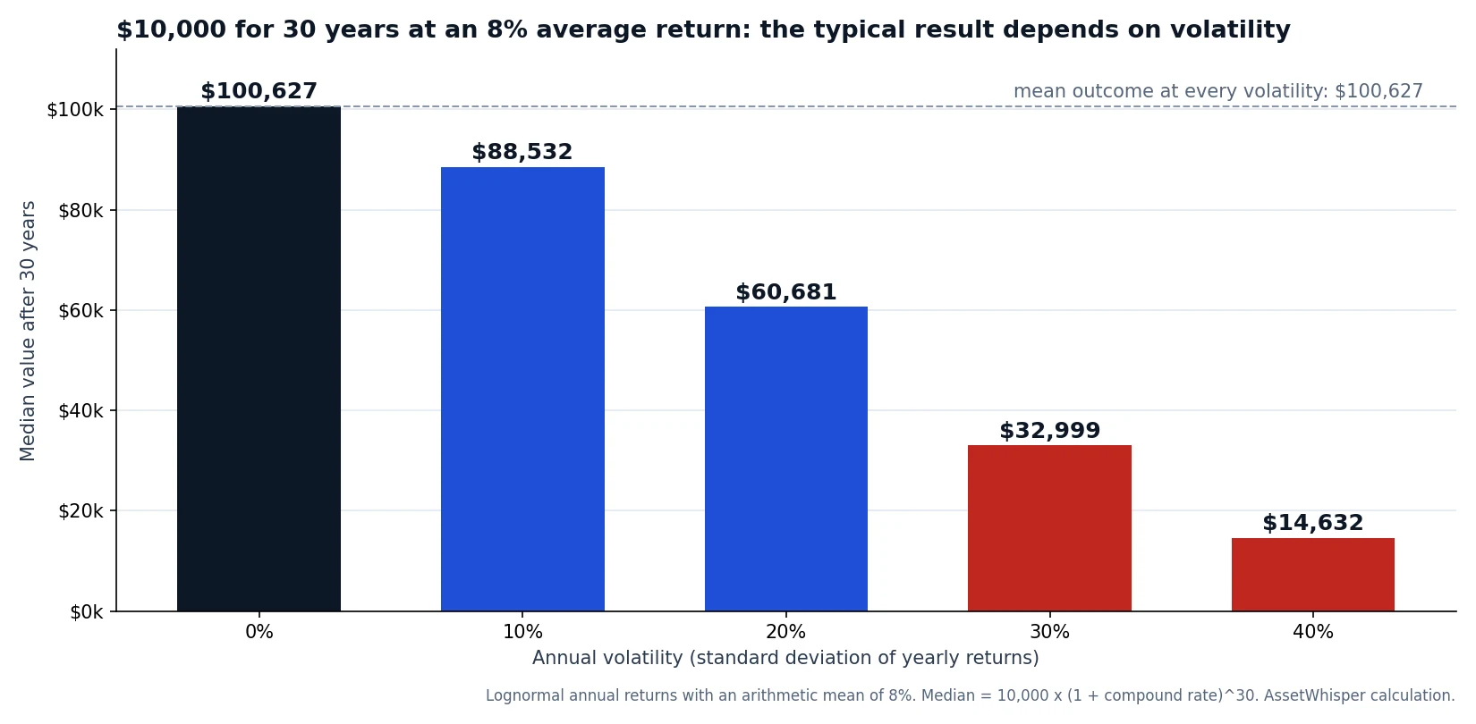
At 20% volatility, close to the S&P 500’s long-run 19.4%, the typical result is $60,681, about 40% below what the average return implies. At 60% volatility, an 8% average return compounds at a loss of 5.59% a year. The half-variance rule holds well up to about 20% and then overstates the drag, because real returns are not symmetric: in the bottom size decile it predicts 7.20 points against an actual gap of 5.79, helped by years like 1933 (+146.6%).
Both averages are right: they answer different questions
If the mean and the median both describe the same investment, which one describes you? We drew 200,000 thirty-year histories at random from the S&P 500’s 98 calendar years, each year picked with replacement, and compounded each one.
- The mean of the 200,000 outcomes was 28.8 times the starting sum, exactly what compounding the 11.85% average for 30 years gives.
- The median was 18.0 times, close to compounding the 10.02% rate (17.5 times).
- Only 32% of the histories reached the outcome implied by the average return. About half reached the one implied by the compound rate.
- The top 10% of histories held 37% of all the wealth across the 200,000. That is what pulls the mean up: a minority of very good histories, not the typical one.
| Horizon | Reaching the average |
|---|---|
| 1 year | 55.2% |
| 5 years | 45.3% |
| 10 years | 40.8% |
| 20 years | 35.8% |
| 30 years | 32.2% |
| 40 years | 29.3% |
The longer the horizon, the further the typical outcome falls behind the average one. Over a single year more than half of outcomes beat the mean, because the distribution of yearly returns has a long left tail. Over 40 years, fewer than three in ten do.
The practical consequence: a projection that compounds an arithmetic average describes the mean of all possible histories, and roughly two in three investors end up below it over 30 years. A projection at the compound rate describes the median, which is a coin flip. Our investment calculator compounds whatever annual rate you type at a constant rate, so the rate to enter is a compound rate, not an average of yearly returns. Neither is a forecast: the 10.02% is what one past century delivered, and starting valuations matter for the next one, as the equity risk premium on CAPE shows.
Leveraged ETFs: the drag, multiplied
A leveraged ETF such as a 2x or 3x S&P 500 fund targets a multiple of the index’s return for one day, and resets its exposure every evening. ProShares states it plainly on its fund pages: for any holding period other than a day, the return “may be higher or lower than the Daily Target”, and “smaller index gains/losses and higher index volatility contribute to returns worse than the Daily Target.”
The reason is the same arithmetic. Tripling the daily return roughly triples the average return, but it multiplies the variance by nine, and with it the drag. On top of that the fund pays to borrow the extra exposure. We simulated daily-reset funds on the S&P 500 from January 1950 to September 2026, dividends included, financed at the Treasury bill rate. In the “with costs” column, each fund also pays a 0.88% annual fee and a financing spread calibrated on the real funds (explained below). “Years under water” counts from the peak before the worst fall to the first close back above it.
| Leverage | Before costs | With costs | Worst fall | Years under water |
|---|---|---|---|---|
| 1x (the index) | 11.66% | 11.66% | −55.3% | 4.5 (Oct 2007 – Apr 2012) |
| 1.5x | 14.54% | 13.11% | −75.1% | 13.3 (Mar 2000 – Jul 2013) |
| 2x | 16.75% | 14.86% | −88.4% | 14.6 (Mar 2000 – Nov 2014) |
| 2.5x | 18.22% | 15.87% | −95.1% | 17.2 (Mar 2000 – Jun 2017) |
| 3x | 18.89% | 16.09% | −98.2% | 19.6 (Mar 2000 – Nov 2019) |
| 4x | 17.55% | 13.92% | −99.8% | 26.1 (Mar 2000 – May 2026) |
The table contains an uncomfortable result, and it is worth stating plainly: over these 76 years, in hindsight, leverage raised the average return by more than the drag took away. A simulated 3x fund compounded at 16.1% after costs against 11.7% for the index. What the drag did was everything else.
- Three times the index is not three times the return. After costs, the 3x fund compounded at less than half of three times the index’s rate (35.0%). Even before costs, in 56 of 76 calendar years it returned less than three times the index. In nine years (1960, 1970, 1978, 1984, 1987, 1994, 2007, 2011 and 2015) the index rose and the 3x fund fell.
- Flat markets are where it shows. In every one of the 1,024 one-year windows in which the index ended within 2% of where it started, the 3x simulation lost money before costs, with a median loss of 11.4% and a worst of 47.7%. (The windows overlap, so they are not 1,024 independent cases, but they span 47 different calendar years.)
- The path was close to total loss. With costs, the 3x fund fell 98.2% from March 2000 to March 2009 and did not regain its 2000 peak until November 2019, 19.6 years later. The 2x fund needed 14.6 years. Over 2000–2012 alone, before costs, the index compounded at 1.6% a year, the 2x fund at −3.4% and the 3x fund at −12.4%.
- One day can end it. On 19 October 1987 the S&P 500 fell 20.45%; a 3x fund would have lost 61.4% in one session, and any daily leverage above 4.89 times would have been wiped out.
Daily resetting also cuts both ways. In 2008, the index’s total return was −37.0% and the 3x simulation lost 85.5%, far less than the 111% that three times the index’s loss would imply, because the fund’s exposure shrank as it fell. In a steady trend, up or down, the reset helps; in a market that swings back and forth, it hurts. The SEC’s investor bulletin on these products gives a real case of the second kind: over four months, a fund targeting three times its index’s daily return fell 53% while the index gained about 8%.
How close is the simulation to real funds? We checked it against ProShares Ultra S&P 500 (SSO, 2x) and ProShares UltraPro S&P 500 (UPRO, 3x), using their adjusted prices with distributions reinvested. All figures are compound annual rates; “simulated” includes each fund’s expense ratio.
| To 30 Sep 2026 | Index | Fund | Simulated | L × index |
|---|---|---|---|---|
| SSO (2x), since June 2006 | 11.44% | 15.65% | 16.58% | 22.87% |
| UPRO (3x), since June 2009 | 15.16% | 32.59% | 34.47% | 45.49% |
Daily returns of the simulation and the real funds correlate at 0.995 (SSO) and 0.998 (UPRO). The remaining shortfall implies that the real funds paid about 0.8 (SSO) and 0.7 (UPRO) points a year above the bill rate on each unit of borrowed exposure, which covers financing and any other tracking costs. Their average, 0.75, is the spread used in the “with costs” column. UPRO was launched about three months after the March 2009 low, at the start of a long bull market, and still compounded at well under three times the index. It lost 76.5% between 19 February and 23 March 2020, when the index lost 33.5%. In 2022 the index lost 18.1%, SSO 39.0% and UPRO 56.8%. Inverse funds suffer the same mechanism in reverse, as we measured in portfolio hedging strategies.
How much leverage maximises growth, and why nobody knows in advance
Leverage adds return in a straight line and drag along a curve, so there is a level where growth peaks. Edward Thorp’s treatment of the Kelly criterion for the stock market gives it in closed form: the growth rate is g = r + f(m − r) − s²f²/2, maximised at f* = (m − r)/s², where m is the average return, r the risk-free rate and s the volatility. It is the continuous version of the betting fraction in our Kelly article. Thorp’s own rough S&P 500 estimates (m = 11%, s = 15%, r = 6%) give f* ≈ 2.2.
| Period | Excess return | Volatility | Formula | Best in data |
|---|---|---|---|---|
| 1950–2026 | 8.24% | 15.74% | 3.32 | 3.15 |
| 1950–1999 | 8.42% | 13.52% | 4.61 | 3.85 |
| 2000–2026 | 7.89% | 19.22% | 2.14 | 2.10 |
| 2000–2012 | 1.83% | 21.43% | 0.40 | 0.40 |
| 2013–2026 | 13.63% | 16.86% | 4.79 | 4.50 |
Daily data, before costs, with the benefit of hindsight. “Formula” is (m − r)/s²; “best in data” is the leverage that actually produced the highest compound rate. With the costs above, the best leverage over 1950–2026 falls to 2.9. The point of the table is the spread: the leverage that maximised growth was 0.4 in one stretch and 4.8 in the next, because it depends on the ratio of excess return to variance, and both move from decade to decade. Choosing a leverage is choosing a forecast of that ratio. Thorp’s formula also implies that at twice the optimum, growth falls back to the risk-free rate, and the continuous model ignores jumps: the 1987 crash alone set a hard ceiling of 4.89 times.
The one place the drag works for you: mixing assets
A portfolio’s average return is the weighted average of its parts’ average returns: 60% of 11.85% plus 40% of 4.82% is 9.04%, exactly the 60/40 figure in the first table. Its volatility is not a weighted average. Stocks and bonds had a correlation of 0.02 in yearly returns over 1928–2025, so the 60/40 portfolio’s volatility was 12.12%, against 14.80% for a weighted average of the two volatilities. Less variance means less drag: 0.70 points, against 1.22 for 60/40 of the two drags.
The result is that the 60/40 compounded at 8.34% a year, 0.52 points above 60% of the stock compound rate plus 40% of the bond compound rate (7.82%). David Booth and Eugene Fama called this the diversification return in 1992. It means that a portfolio’s compound return cannot be estimated by averaging its holdings’ compound returns.
It does not mean rebalancing beats leaving the portfolio alone. A 60/40 that was never rebalanced compounded at 9.45% over the same years, because by 2025 it had drifted to 99.6% stocks and was a different portfolio. Rebalancing keeps the risk you chose, a point developed in how often to rebalance.
What this changes
- Reading a return figure. When a return is quoted as an “average annual return”, check whether it is the arithmetic mean of yearly returns or the annualised compound rate. Only the second tells you what the money did. Our calculator’s Returns tab gives the compound rate (CAGR) from a start and end value.
- Making a projection. Use a compound rate, and remember it is a median: half of the outcomes are worse.
- Comparing two investments with the same average return. The less volatile one compounds faster. This is part of why return per unit of risk, such as the Sharpe ratio, matters beyond comfort.
- Holding a leveraged product for longer than a day. The outcome depends on the path and on the ratio of return to variance over the holding period, not on the multiple printed on the fund. Sizing leverage is the same problem as position sizing and the risk of ruin.
What this does not say
- Not that low volatility is better. Bonds had a drag of 0.29 points and still compounded at 4.53% against 10.02% for stocks. The drag is a cost measured against an asset’s own average return, not a ranking of assets.
- Not that leveraged ETFs always lose. In this simulation, 3x compounded faster than the index over 1950–2026 after costs, and UPRO has since 2009. What the data shows is that the result depends on an unknowable ratio and comes with paths that lose almost everything.
- Not a forecast. The historical compound rate of 10.02% is what one past century delivered, not an expected return.
- Not exact. Half the variance is an approximation; it overstates the drag for very volatile, right-skewed assets. The figures above are computed directly, not from the rule.
Frequently asked questions
What is volatility drag?
It is the gap between the arithmetic average of a series of returns and the compound rate those returns actually produce. It exists because losses need larger gains to recover. For the S&P 500 over 1928–2025 the average yearly return was 11.85% and the compound rate 10.02%, a gap of 1.84 points.
How do you calculate volatility drag?
Directly, by subtracting the compound rate from the arithmetic mean of the same returns. As an approximation, it is about half the variance: half the square of the volatility. With the S&P 500’s yearly volatility of 19.40%, the approximation gives 1.88 points against an actual 1.84.
Which return should I use to project my portfolio?
A compound rate, because it describes the median outcome. Compounding the arithmetic average gives the mean outcome, which in our resampling of S&P 500 history only about 32% of 30-year histories reached. Neither number is a forecast of future returns.
Why do leveraged ETFs lose value even when the index goes up?
Because they reset to their target leverage every day, which multiplies the variance, and with it the drag, by the square of the leverage, and because they pay to borrow. In our 1950–2026 simulation, a 3x S&P 500 fund lost money, before costs, in all 1,024 one-year windows in which the index ended within 2% of its start, and fell in nine calendar years in which the index rose.
Does diversification reduce volatility drag?
Yes, when the assets are not perfectly correlated. A 60/40 stock and bond portfolio rebalanced yearly compounded at 8.34% over 1928–2025, 0.52 points more than 60/40 of the two assets’ compound rates, because its volatility was lower than the average of theirs.
Does the order of returns matter?
Not for a single sum with no additions or withdrawals: multiplication does not depend on order, so the same returns in any sequence give the same compound rate. Order matters when money flows in or out, which is the sequence risk we measured for retirement withdrawals in the 4% rule.
How we calculated this
- Yearly returns: Damodaran’s historical returns spreadsheet (updated January 2026), calendar years 1928–2025: S&P 500 with dividends, 10-year Treasury bond, 3-month Treasury bill and bottom-decile US stocks. Average = simple mean; compound rate = (product of 1 + return)1/n − 1; volatility = sample standard deviation. Damodaran’s own summary gives the same 11.85% and 10.02% for the S&P 500.
- Small stocks: the bottom-decile series matches Kenneth French’s value-weighted bottom decile of US stocks by market value (correlation 1.000; compound rate 12.00% against 11.98%). Damodaran’s spreadsheet prints a geometric average of 0.16% for this series because its cumulative-value column restarts every year; compounding the yearly returns gives 11.98%.
- 60/40: 60% S&P 500, 40% 10-year Treasury, reset every January; the never-rebalanced version starts at 60/40 in 1928 and is left alone.
- Volatility table: lognormal yearly returns with an arithmetic mean of 8%; compound rate = 1.08 / √(1 + σ²/1.08²) − 1; median 30-year value = $10,000 × (1 + compound rate)30; mean = $10,000 × 1.0830.
- Resampling: 200,000 thirty-year paths drawn with replacement from the 98 S&P 500 calendar years. This treats years as independent, which ignores valuation and mean reversion.
- Leverage simulation: daily S&P 500 closes (^GSPC), 3 January 1950 to 30 September 2026, plus 1/252 of Shiller’s dividend yield per session (11.41% a year against 11.47% for the official total-return index over 1988–2026). Fund return each day = L × index return − (L − 1) × financing − fee/252, floored at −100%. Financing: the 13-week Treasury bill rate (^IRX) from 1960, Damodaran’s T-bill return for 1950–1959. “With costs” adds a 0.88% fee (the average of SSO’s 0.87% and UPRO’s 0.89% net expense ratios) and a 0.75% spread on borrowed exposure, the average of the spreads that make the simulation match SSO and UPRO. No taxes or trading spreads.
- Growth-optimal leverage: formula from annualised daily excess returns and variance; “best in the data” is the leverage, in steps of 0.05 from 0 to 6, with the highest compound rate.
- Limits: one market, one historical path, and simulated funds for every year before 2006. The script that prints every figure in this article is kept with its working files.
Sources
- Aswath Damodaran, Historical Returns on Stocks, Bonds and Bills (spreadsheet), NYU Stern, updated 1 January 2026.
- Kenneth R. French, Data Library: Portfolios Formed on Size, annual returns.
- Robert J. Shiller, U.S. Stock Markets 1871–Present and CAPE Ratio (dividends and price).
- Yahoo Finance: ^GSPC, ^SP500TR and ^IRX daily data; SSO and UPRO adjusted closes.
- ProShares, fund pages for UPRO and SSO: daily objectives, inception dates and expense ratios, accessed 4 October 2026.
- U.S. Securities and Exchange Commission, Office of Investor Education and Advocacy, Updated Investor Bulletin: Leveraged and Inverse ETFs, 29 August 2023.
- Edward O. Thorp, The Kelly Criterion in Blackjack, Sports Betting, and the Stock Market, chapter 9 in Handbook of Asset and Liability Management, vol. 1, Elsevier, 2006. Section 7.1, equations 7.2 and 7.3, and example 7.2.
- David G. Booth and Eugene F. Fama, “Diversification Returns and Asset Contributions”, Financial Analysts Journal, 48(3), 1992.
Related reading
- Compound interest: how much of the final sum was ever yours — the compounding this article puts a volatility discount on.
- The Kelly criterion, and why nobody runs full Kelly — the same growth-versus-variance trade-off, for bet sizing.
- Portfolio hedging strategies: what each one costs — inverse ETFs and the daily reset.
- Bear markets since 1950 — how long the losses that drive the drag took to recover.
- Risk parity and volatility targeting — two strategies that use leverage to manage risk, tested from 1965 to 2026.
This article is general information, not personalised investment advice. It does not take into account the financial situation, objectives, tax position or risk tolerance of any individual reader, and the same text is distributed to all readers. Historical and simulated results describe the past under stated assumptions and are not forecasts. Leveraged and inverse funds are complex products that can lose most or all of their value, and their returns over periods longer than one day can differ greatly from their stated multiple. Capital is at risk.