How Much Risk Does Diversification Remove? 48 US Industries, 1969–2026
Key takeaway
From 1969 to 2026 the average US industry had 23.2% annual volatility. Ten industries chosen at random cut it to 17.8% and all 48 to 17.2%, but diversification did not protect against the market’s own fall: weighted by value, the 48 industries lost within 1.3 points of the market in six falls of more than 20%.

“Don’t put all your eggs in one basket” is among the most repeated sentences in investing, and the advice that repeats it rarely shows the numbers. How much risk does the second basket remove? The tenth? Is there a point after which holding more adds nothing, and what is left when it does? We put numbers on those questions with Kenneth French’s industry portfolios. Every June, his data library assigns the US stocks in the CRSP database (NYSE, AMEX and Nasdaq) to 49 industries by SIC code and records what each industry returned month by month; the series starts in July 1926. We dropped the library’s 49th group, “Other”, which is a catch-all rather than an industry, and, because nine of the remaining industries only enter the data after 1926 (healthcare, the last, in July 1969), we used the complete 48-industry panel: July 1969 to September 2026, 687 months.
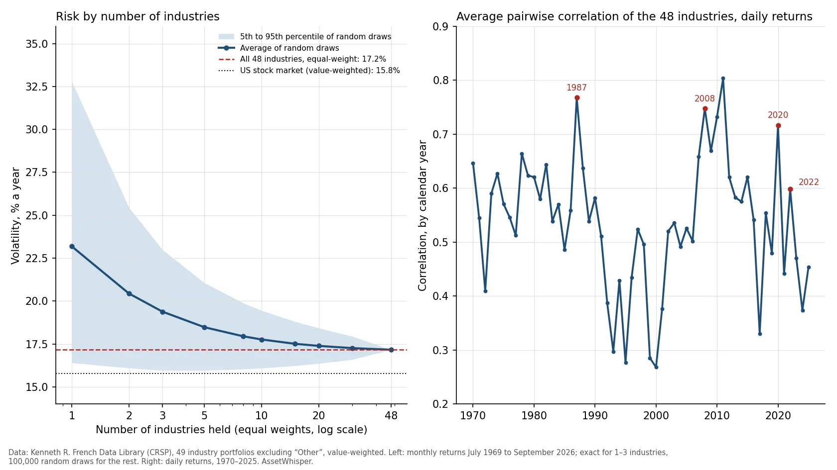
Holding one US industry meant 23.2% volatility a year on average from 1969 to 2026. Ten randomly chosen industries cut it to 17.8%, and all 48 to 17.2%, so the first ten did 90% of the work. What was left was market risk: the 48-industry portfolio fell 52.4% in 2007–09, the market 50.3%.
The short answer, in one table
For each number of industries, we took every possible combination (one, two and three industries) or drew that many industries at random 100,000 times (the rest), held them in equal weights, rebalanced every month, before trading costs and taxes, and measured each portfolio over the 57 years. Volatility is the average across the portfolios, return and worst fall are medians, and the 5th–95th range shows how much the answer depended on luck. “Share of the fall” is how much of the drop in volatility between one industry and all 48 had been achieved. The last row is the whole US stock market, value-weighted.
| Industries held | Volatility | 5th–95th | Share of the fall | Median return | Median worst fall |
|---|---|---|---|---|---|
| 1 | 23.2% | 16.4%–32.8% | 0% | 10.11% | −66.7% |
| 2 | 20.4% | 16.1%–25.4% | 46% | 10.55% | −60.6% |
| 3 | 19.4% | 16.0%–23.0% | 63% | 10.77% | −58.4% |
| 5 | 18.5% | 16.0%–21.1% | 78% | 10.94% | −56.2% |
| 10 | 17.8% | 16.1%–19.4% | 90% | 11.08% | −54.2% |
| 20 | 17.4% | 16.4%–18.4% | 96% | 11.15% | −53.0% |
| All 48 | 17.2% | – | 100% | 11.20% | −52.4% |
| US market | 15.8% | – | – | 10.94% | −50.3% |
The curve is steep at the start and flat at the end. Going from one industry to two removed 46% of everything the 48 together removed; five industries took it to 78%; ten, to 90%. Between 20 industries and 48, volatility moved from 17.4% to 17.2%. Two other things in the table matter as much as the average. The range of outcomes narrows fast: nine times out of ten a single industry had a volatility between 16.4% and 32.8%, and five industries between 16.0% and 21.1%. And in this sample diversification did not cost return: the median compound return went up with every industry added, from 10.11% to 11.20%, for reasons the third section explains. That return is before trading costs, and the 48-industry portfolio also compounded above the market (11.20% against 10.94%) for a reason that has more to do with weighting than with the number of industries: the same 48 industries weighted by market value compounded 11.13%.
What diversification removes: the part that belongs to the industry
Single industries were far from the market’s 15.8%. The average industry had a volatility of 23.2%, from 14.4% for utilities to 38.9% for coal, and 46 of the 48 industries were more volatile than the market. In their worst falls the industries lost a median of 66.7% from peak to trough (the median of the 48); coal lost 98.7%, and only four of the 48 had a smaller worst fall than the market’s 50.3%.
Part of that is the market, which no industry escapes, and part belongs to the industry. Regressing each industry’s monthly returns on the market’s, the market explained a median 56% of an industry’s variance, from 6% for precious metals to 83% for business services. The other 44% (the median) is what the market does not explain: it includes the industry’s own commodity prices, regulation and technology cycle, and any tilt to small or value stocks; we did not split it. The part that is specific to each industry does not move with the others, and that is the part that cancels when industries are combined; a shared tilt to small or value stocks does not. Harry Markowitz set out the logic in 1952, and he named industries: “It is necessary to avoid investing in securities with high covariances among themselves. We should diversify across industries because firms in different industries, especially industries with different economic characteristics, have lower covariances than firms within an industry.”
The result is visible in the portfolio of all 48. Its volatility of 17.2% corresponds to a variance of 0.0295, against an average of 0.0563 for a single industry: diversifying across all 48 removed 48% of the typical industry’s variance. The market explained 91% of the 48-industry portfolio’s variance (beta 1.04 in a regression on the market alone, correlation 0.96), against 56% for the typical industry. What was left was almost entirely the thing the market is made of.
Notice that the floor, 17.2%, sits above the market’s 15.8%, and the reason is weighting: equal weights give coal or gold, small and volatile industries, the same weight as the largest ones, and the value-weighted market does not. Weighted by market value, the same 48 industries had a volatility of 15.7%, and the equal-weight portfolio carries a tilt to small and value stocks (loadings of 0.20 on each of the Fama-French size and value factors). The floor is the risk of owning US industries evenly, not zero risk.
What it added: a higher compound return in this sample
The median return in the table rose from 10.11% with one industry to 11.20% with 48, and nothing about the industries’ average return changed. Take the arithmetic mean of monthly returns, times 12: it was 12.15% for the average industry and exactly 12.15% for the equal-weight portfolio of all 48, because the mean of a portfolio is the mean of its parts. The compound rate is different:
| Portfolio | Mean return | Compound return | Variance |
|---|---|---|---|
| Average single industry | 12.15% | 9.76% | 0.0563 |
| All 48, equal-weight | 12.15% | 11.20% | 0.0295 |
| Difference | 0.00 | +1.44 points | −0.0269 |
The gap between mean and compound return is the volatility drag we measured in our study of volatility drag, and the usual approximation puts it at half the variance. Half of the 0.0269 fall in variance (computed before rounding the two variances shown) is 1.34 points a year, close to the 1.44 measured. The approximation is not exact in each portfolio: it overstates the gap between mean and compound return by about half a point in the average industry (2.82 points against 2.39 measured) and in the 48-industry portfolio (1.47 against 0.95), so the errors largely cancel in the difference. David Booth and Eugene Fama called this extra compound return the diversification return in 1992. Combining industries did not make any of them earn more. It lowered the variance, and the portfolio compounded closer to its average. Two cautions. The result needs a rebalance every month back to equal weights, which has trading costs this test leaves out. And it is one sample: the 9.76% of the average single industry is an average over industries that did very differently for reasons of their own, from real estate at 4.6% a year to tobacco at 15.8%.
Why it stops at 17%: correlation sets the floor
The average correlation between two of the 48 industries’ monthly returns was 0.55, and 0.54 using daily returns. With that much common movement, adding industries makes the portfolio less like any one of them but not like a different asset. With equal variances and an average correlation ρ, the variance of an equal-weight portfolio of N holdings is σ²[1/N + (1 − 1/N)ρ], so it behaves like N / (1 + (N − 1)ρ) independent holdings:
| Average correlation | Independent bets |
|---|---|
| 0.30 | 3.2 |
| 0.55 (measured, 1969–2026) | 1.8 |
| 0.70 | 1.4 |
| 0.90 | 1.1 |
At the measured correlation, 48 US industries behaved like fewer than two independent bets. The direct measure agrees: the average single-industry variance divided by the 48-industry portfolio’s variance is 1.91. That is why the first few holdings do almost all the work and the next forty add little. It is also why the floor can only fall if the holdings are less alike, in industries, countries or asset classes. Our look at the 60/40 portfolio and our test of risk parity deal with what happens when bonds are added to stocks. This study stays inside one asset class and measures how little industry labels do.
In six market falls: when diversification helped and when it did not
The question investors ask is not about average volatility but about what happens in a crash. The table takes each of the six falls of more than 20% in the US market that began after July 1969 (peak and trough month-ends of the market itself) and shows what the portfolio of all 48 industries did, in equal weights and weighted by market value, and how far apart the industries were. These falls use month-end total returns of the CRSP value-weighted market, so they are shallower than the daily-price falls in our study of bear markets (−56.8% for 2007–09, about −34% for the 2020 crash), and the 2020 fall clears the 20% threshold on month-end data by only 0.2 points. A seventh fall, November 1968 to June 1970 (−33.6%), began before the panel and is not in the table; over its last twelve months inside the panel (July 1969 to June 1970) the market lost 25.6% and the equal-weight portfolio 30.1%.
| Fall | Market | 48 equal | 48 by value | Best industry | Worst industry | Up |
|---|---|---|---|---|---|---|
| Dec 1972–Sep 1974 | −46.5% | −48.1% | −45.2% | Precious metals +34.3% | Healthcare −80.4% | 1 |
| Aug–Nov 1987 | −29.9% | −31.3% | −29.7% | Utilities −11.4% | Apparel −44.3% | 0 |
| Aug 2000–Sep 2002 | −45.0% | −15.4% | −43.8% | Defense +135.1% | Computers −84.3% | 21 |
| Oct 2007–Feb 2009 | −50.3% | −52.4% | −49.4% | Agriculture −24.1% | Entertainment −80.4% | 0 |
| Jan–Mar 2020 | −20.2% | −24.6% | −20.2% | Precious metals −3.2% | Coal −46.1% | 0 |
| Dec 2021–Sep 2022 | −24.8% | −20.8% | −24.6% | Coal +80.1% | Recreation −53.7% | 5 |
“Up” counts the industries, out of 48, with a positive return between the market’s peak and trough. “48 equal” is all 48 industries in equal weights, rebalanced monthly; “48 by value” weights the same industries by their market value (number of firms times average firm size at the start of each month). Returns are total returns of value-weighted industry portfolios.
In four of the six falls the equal-weight portfolio of all 48 industries lost 1.5 to 4.4 points more than the market (48.1%, 31.3%, 52.4% and 24.6%); in two it lost less (20.8% against 24.8% in 2021–22 and 15.4% against 45.0% in 2000–02). Averaged over the six, it lost 32.1% against the market’s 36.1%. Most of that difference comes from weighting, not from the number of industries: the same 48 industries weighted by market value lost within 1.3 points of the market in every fall. Holding more industries did not protect against the market’s own fall. In 2007–09 every one of the 48 fell. The spread between the best and the worst industry was 56 points, and a random ten-industry portfolio lost a median of 52.4%, with a 5th-to-95th percentile range of 44.6% to 59.7%. Diversification narrowed the range around the market’s loss; it did not move it. The same was true further back. From August 1929 to June 1932, in the 39 industries that have data for the whole century, the market lost 83.7%, the equal-weight portfolio 85.3%, and all 39 industries fell, from 44.1% for tobacco to 95.7% for real estate.
The dot-com bust is the exception, and it is an exception of weighting. The market lost 45.0% from August 2000 to September 2002, but the equal-weight portfolio lost 15.4%, and 21 of the 48 industries rose. Computers and electronic equipment lost about 84% each, while defense, precious metals and tobacco went up. At the end of August 2000 software, electronic equipment and computers were about a third of the US market’s value (33%: 12.4%, 11.0% and 9.4%), against 6% of the equal-weight portfolio, and by September 2002 they had lost 73%, 84% and 84%. Weighting the same 48 industries by market value gives a fall of 43.8%, close to the market’s 45.0%. The three best industries, defense, precious metals and tobacco, held 7, 7 and 5 stocks each at the end of August 2000, so part of the equal-weight result rests on very few companies. In calendar 2000 the best industry (coal) gained 104.4% and the worst (software) lost 50.3%, a spread of 155 points.
The falls also show how much the answer depends on which industries are held. In 2007–09 a random ten-industry portfolio lost between 44.6% and 59.7% (5th to 95th percentile), a 15-point range around the same market. Average-volatility numbers hide that range; for how long the recoveries took, see our study of bear markets.
Do correlations rise when markets fall?
In three of the six stress windows we checked the average correlation was well above the long-run level, in two it was barely above it, and in one it was below it. The average correlation between pairs of the 48 industries, from daily returns, ran from 0.27 in 2000 to 0.80 in 2011; it was 0.75 in 2008, 0.72 in 2020 and 0.60 in 2022, against a long-run average of 0.54. The highest year, 2011, had no fall of more than 20% at month-end (the deepest was 17.7%), but on daily data the market fell 20.3% from 29 April to 3 October 2011, and the average correlation in that window was 0.84, the same as in 1987. Measured over the stress windows themselves, the figure was 0.84 for the crash of October to early December 1987, 0.74 from October 2007 to March 2009 and 0.81 for the 24 trading days of the February–March 2020 fall; it was 0.60 in the 1973–74 bear market and 0.59 from January to mid-October 2022, small rises. The dot-com bust fell the other way: 0.37 over the 638 trading days from March 2000 to October 2002, and 0.40 over the 520 trading days between the dates of the falls table. The first five months of that window were a flat market (−3.1%) with an average correlation of 0.24; we did not test why it was so low. Four of the windows (1973–74, 2000–02, 2007–09 and February–March 2020) run from the CRSP market’s own daily peak to its daily trough. The other two use the S&P 500 dates of our bear-market study (1 October to 4 December for 1987, 3 January to 12 October for 2022); measured from the CRSP market’s own daily peaks (25 August 1987 and 8 November 2021) the correlations are 0.83 and 0.58. The windows differ slightly from the month-end dates in the table above and range from 24 to 638 trading days. Some of our earlier articles describe correlations in a crisis as converging toward one; in these data they rose clearly in three of the six windows and were never close to one.
Sorting quarters from calmest to most volatile, by the market’s own daily volatility, gives the same story without reference to any particular crisis. In the calmest 25% of quarters the average correlation was 0.43, in the most volatile 25% it was 0.60.
| Quarters since 1969, by market volatility | Market volatility | Average correlation |
|---|---|---|
| Calmest 25% of quarters | 8.7% | 0.43 |
| Second | 11.4% | 0.52 |
| Third | 14.5% | 0.53 |
| Most volatile 25% | 24.8% | 0.60 |
One caution in reading this. Kristin Forbes and Roberto Rigobon showed in 2002 that correlation coefficients are conditional on market volatility: when volatility rises, measured correlations rise with it. In their tests across national stock markets, and under certain assumptions, adjusting for that removed virtually all of the apparent increase in correlation in the 1987 crash, the 1994 Mexican devaluation and the 1997 Asian crisis. We did not make that adjustment, and their tests are for countries, not industries within one market, so the figures above are as measured. They describe what an investor holding these industries lived through, which was a much higher correlation in 1987, 2008 and 2020 than on average, a little higher in 1973–74 and 2022, and a lower one in 2000–02; they do not show why.
Industries are not stocks
This study does not say how many stocks are enough, and the industry result should not be read as if it did. Each of French’s industry portfolios is already a basket of stocks, but not always a big one. In July 1969 the median industry portfolio held 30 or 31 stocks and the smallest held one; in September 2026 the median held 41 and the smallest 4 (fabricated products), with 15 of the 48 under 20 stocks. Coal had 3 stocks in July 2000 and 6 in September 2026, and gold had 5 in June 2009. Some of the volatility of those industries, coal at 38.9% and gold at 37.2%, is therefore company-specific, and for the same reason the single-industry numbers here understate what one stock would have shown.
The literature on individual stocks gives larger numbers than ours. Meir Statman argued in 1987 that a well-diversified portfolio of randomly chosen stocks must include at least 30 stocks for an investor who borrows and 40 for one who lends, and that this contradicts the widely held view that the benefits are virtually exhausted at about 10 stocks. John Campbell, Martin Lettau, Burton Malkiel and Yexiao Xu found that between 1962 and 1997 firm-level volatility rose relative to market volatility, and that, accordingly, correlations among individual stocks fell and the number of stocks needed to achieve a given level of diversification increased. Our result is not in conflict: ten industries were enough to get 90% of the reduction in risk that 48 provide, but ten industries typically means several hundred stocks.
What the evidence supports, and what it does not
- It supports: combining US industries removes risk quickly at first: 78% of the available fall in volatility with five industries, 90% with ten, 96% with twenty, in 57 years of data. The volatility falls from 23.2% to 17.2%, and variance by about half.
- It supports: diversification raised the compound return, with the same average return, by about 1.1 to 1.4 points a year (1.09 for the median industry portfolio, 1.44 for the average one), through lower volatility drag, assuming monthly rebalancing and no costs, in this sample.
- It does not support: the claim that holding many industries protects against a market-wide fall: what the portfolio lost depended on its weighting more than on the number of industries. In four of six falls over 20% the equal-weight 48-industry portfolio lost 1.5 to 4.4 points more than the market, in two it lost less, and a value-weighted version of the same 48 industries lost within 1.3 points of the market in all six; in 2007–09 and 1929–32 every industry fell.
- It does not support: a rule that correlations always jump in a crash. They were far higher in 1987, 2008 and 2020, only a little higher in 1973–74 and 2022, and lower than average in 2000–02.
- It cannot say: how many individual stocks are enough, whether the next decades will look like these 57 years, or what an investor with other assets, costs or taxes would have experienced.
For the broader question of what an investor can do about market risk itself, see our guide to managing risk, and our comparison of hedging strategies and their costs for what it costs to hold less of it. To try other weights or return assumptions, use the investment calculator.
Frequently asked questions
How many industries do you need to diversify a stock portfolio?
In US data from July 1969 to September 2026, five randomly chosen industries achieved 78% of the fall in volatility that all 48 achieved, ten achieved 90% and twenty 96%. Volatility fell from 23.2% for one industry to 17.8% for ten and 17.2% for 48. This counts industries, not stocks: the literature on individual stocks finds that more holdings are needed.
Does diversification protect a portfolio in a crash?
Against the part of a fall that belongs to one industry, yes; against the market’s own fall, little. In 2007–09 the market lost 50.3% and the equal-weight portfolio of all 48 industries lost 52.4%, with every industry down. Over six market falls of more than 20% it lost 32.1% on average against the market’s 36.1%, but the same 48 industries weighted by market value lost within 1.3 points of the market in each one. The 2000–02 bust shows the difference: the equal-weight portfolio lost 15.4% against 45.0% for the market, with 21 industries up, because equal weights held far less of the software, electronics and computer industries that fell most; weighted by value, the 48 industries lost 43.8%.
Do correlations rise in a crash?
Often, but not always. The average correlation between the 48 industries was 0.84 in the 1987 crash, 0.74 in 2007–09 and 0.81 in early 2020, against 0.54 on average; only slightly higher in 1973–74 (0.60) and 2022 (0.59); and 0.37 in the 2000–02 bust. Forbes and Rigobon showed, under stated assumptions, that part of any rise in measured correlation comes from higher volatility itself.
Does diversification reduce returns?
Not in this sample. The average return stayed at 12.15% a year, and the compound return rose from 9.76% for the average industry to 11.20% for the 48-industry portfolio, because lower volatility means less volatility drag. The result assumes monthly rebalancing to equal weights and ignores trading costs.
Why does adding more holdings eventually stop helping?
Because of correlation. The 48 industries had an average correlation of 0.55, which makes them behave like fewer than two independent bets. The common part is market risk, and no number of industries removes it.
How we calculated this
- Data: Kenneth R. French Data Library, “49 Industry Portfolios” (value-weighted, monthly and daily) and “Fama/French 3 Factors” (monthly and daily), built from the CRSP database of September 2026. The industries are defined by the library from SIC codes; “Other” (almost nothing) is excluded. The market is the Mkt-RF plus RF series: all CRSP firms incorporated in the US and listed on the NYSE, AMEX or Nasdaq (share codes 10 and 11), value-weighted. “49 Industry Portfolios” is not the library’s separate “48 Industry Portfolios” file; with that file the results are almost the same (volatility 23.0% for one industry and 17.0% for all). Nine industries enter the data between 1927 and 1969, so every test uses the complete 48-industry panel, July 1969 to September 2026 (687 months; daily: 14,434 days, one day with a missing industry value being excluded), except the 1929–32 line, which uses the 39 industries with data for the whole of July 1926 to September 2026.
- Random portfolios: for N = 1, 2 and 3, every possible combination of N industries (48, 1,128 and 17,296); for N = 5, 8, 10, 15, 20 and 30, 100,000 random draws of N industries without replacement (seed 20261029); equal-weight, rebalanced monthly; N = 48 is the single portfolio of all. Volatility is the standard deviation of monthly returns × √12; return is the compound annual rate; worst fall is the largest month-end peak-to-trough fall. The table shows the mean (volatility) or the median (return, fall) across draws.
- Variance and R²: annualised variance = volatility squared. R² and beta from a regression of each industry’s monthly return on the market’s. The equal-weight 48-industry portfolio has a market beta of 1.03 (1.04 in a regression on the market alone) and loadings of 0.20 on the size and value factors (monthly regression on the Fama-French three factors).
- Value-weighted version: the 48 industries weighted by their market value, number of firms times average firm size from the same file, at the start of each month (French’s file labels each month with the value at the end of the previous month) and rebalanced monthly; its correlation with the market is 0.999. The industry weights at the end of August 2000 are the September 2000 row of the same file. Weighting with the previous month’s values instead moves the value-weighted falls by at most 0.3 points.
- Correlation: the average of all pairwise Pearson correlations between the 48 industries, monthly (whole panel) and daily (by calendar year, by stress window and by quarter; quarters with fewer than 55 trading days excluded, and 2026 left out of the yearly series because it is incomplete). The stress windows use trading dates from the daily data; four run from the market’s own daily peak to its daily trough and two (1987 and 2022) use the S&P 500 dates of our bear-market study, with the market’s own daily peaks giving 0.83 and 0.58. The “effective bets” formula assumes equal variances.
- Falls: the market’s drawdowns of more than 20% are identified on the month-end value of the CRSP value-weighted market since 1926; the six in this table are the ones whose peak falls inside the 48-industry panel; a seventh, 1968–70, began before it. Industry returns run from the peak month-end to the trough month-end.
- Limits: US stocks only, industry portfolios and not stocks; no taxes, trading costs or fees; equal weights and monthly rebalancing are choices, and a different rule would give different numbers; industries in the library are re-formed each June, so the portfolios are not fixed sets of companies; one historical path. Past returns are not a forecast. The script that prints every figure and draws the chart is kept with this article’s working files.
Sources
- Harry Markowitz, “Portfolio Selection”, Journal of Finance, 7(1), 1952, pp. 77–91 (the passage quoted is on p. 89).
- David G. Booth and Eugene F. Fama, “Diversification Returns and Asset Contributions”, Financial Analysts Journal, 48(3), 1992, pp. 26–32.
- Meir Statman, “How Many Stocks Make a Diversified Portfolio?”, Journal of Financial and Quantitative Analysis, 22(3), 1987, pp. 353–363.
- John Y. Campbell, Martin Lettau, Burton G. Malkiel and Yexiao Xu, “Have Individual Stocks Become More Volatile? An Empirical Exploration of Idiosyncratic Risk”, Journal of Finance, 56(1), 2001, pp. 1–43.
- Kristin J. Forbes and Roberto Rigobon, “No Contagion, Only Interdependence: Measuring Stock Market Comovements”, Journal of Finance, 57(5), 2002, pp. 2223–2261.
- Data: Kenneth R. French, Data Library (49 Industry Portfolios; Fama/French 3 Factors; industry definitions in Siccodes49), CRSP database of September 2026. Retrieved 29 October 2026.
Related reading
- How to manage risk in your financial investments — the broad guide this study measures one part of.
- Volatility drag: why the average return is not the return you get — the arithmetic behind the 1.1-to-1.4-point gap.
- Is 60/40 still alive? — what happens when the second basket is bonds.
- Crisis-proof investments: resilient sectors in times of volatility — what defensive sectors did in four of the same falls.
- Position sizing and risk of ruin — how much to hold of any one thing, as arithmetic.
This article is general information, not personalised investment or tax advice. It does not take into account the financial situation, objectives, tax position or risk tolerance of any individual reader, and the same text is distributed to all readers. Historical and simulated results describe the past under stated assumptions and are not forecasts. Taxes, trading costs and fund fees reduce returns. Capital is at risk.