Does Momentum Investing Work? 99 Years of US Data, Including the Crashes
Key takeaway
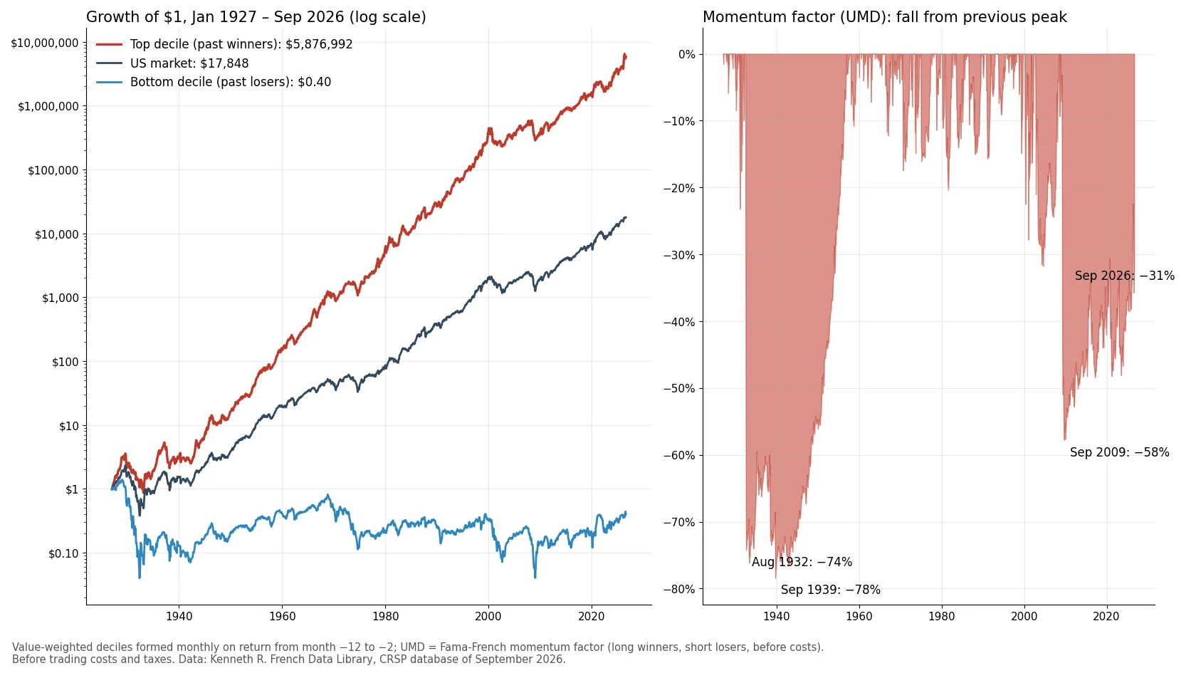
From 1927 to September 2026, the tenth of US stocks with the best past year returned 16.9% a year before costs, against 10.3% for the market. Winners minus losers earned 7.4% a year, but lost 74% in July–August 1932, 58% in 2008–09, and has not regained its November 2008 peak.

Momentum is one of the oldest ideas in technical analysis turned into a rule you can test: stocks that went up over the past year tend to keep going up for a few more months, and stocks that went down tend to keep going down. In our comparison of technical and fundamental analysis we called it a technical idea expressed as a testable rule. This article runs the test. We used Kenneth French’s data library, which every month sorts all US stocks in the CRSP database (NYSE, AMEX and Nasdaq) by their return from twelve months ago to one month ago and splits them into ten groups. The series runs from January 1927 to September 2026: 1,197 months.
From 1927 to September 2026, the tenth of US stocks with the best past year returned 16.9% a year before costs, against 10.3% for the market. Winners minus losers earned 7.4% a year, but lost 74% in July–August 1932, 58% in 2008–09, and has not regained its November 2008 peak.
The short answer, in one table
Each row is one tenth of the market by past return, from the stocks that fell most over months −12 to −2 (decile 1) to those that rose most (decile 10). Each group is weighted by market value and re-formed every month. The return is the compound annual rate before trading costs and taxes; volatility is the annualised standard deviation of monthly returns; the Sharpe ratio is the average return above the one-month Treasury bill divided by volatility. The breakpoints are NYSE deciles, so the groups do not hold equal numbers of stocks: in September 2026 the losers’ decile held 718 stocks and the winners’ 429, of 3,154.
| Decile | Return | Volatility | Sharpe | $1 became |
|---|---|---|---|---|
| 1 (losers) | −0.9% | 33.9% | 0.04 | $0.40 |
| 2 | 5.4% | 27.8% | 0.21 | |
| 3 | 7.1% | 23.8% | 0.27 | |
| 4 | 8.9% | 21.8% | 0.35 | |
| 5 | 9.7% | 20.2% | 0.40 | |
| 6 | 10.3% | 19.8% | 0.43 | |
| 7 | 11.1% | 18.7% | 0.48 | |
| 8 | 12.5% | 18.3% | 0.56 | |
| 9 | 12.9% | 19.1% | 0.56 | |
| 10 (winners) | 16.9% | 22.6% | 0.67 | $5.9 million |
| Market | 10.3% | 18.4% | 0.45 | $17,848 |
The pattern is close to monotonic: every step up in past return comes with a higher later return, from −0.9% to 16.9%. With equal weights instead of value weights the ranking is the same (4.2% for losers, 19.1% for winners). That regularity, across nearly a century and a sample that ends 33 years after the effect was published, is why momentum is one of the most studied and most replicated anomalies in the academic literature.
The $5.9 million is not a result anyone could have achieved. The winners’ decile changes a large part of its holdings every month, and the figure is before trading costs, taxes and fees; the cost section below shows what costs do to the premium.
Winners minus losers: the premium and its size
Researchers measure momentum as a long-short portfolio: buy the winners, sell short the losers, so that the market’s own moves largely cancel out. French publishes a standard version, the momentum factor that Mark Carhart added to the Fama-French model in 1997 (often called UMD, “up minus down”), built from the top and bottom 30% of stocks by past return within large and small companies. It is less extreme than the decile spread because it uses wider groups.
| Long-short | Mean/yr | t-stat | Volatility | Sharpe |
|---|---|---|---|---|
| Decile 10 − 1 | 13.8% | 4.98 | 27.7% | 0.50 |
| Momentum (UMD) | 7.4% | 4.55 | 16.3% | 0.46 |
| Value (HML) | 4.2% | 3.42 | 12.3% | 0.34 |
| Market − T-bill | 8.3% | 4.50 | 18.4% | 0.45 |
Over the whole period, the momentum factor’s average premium was about as large and as reliable as the equity premium itself. It is also not explained by the usual risk factors. Regressed on the Fama-French three factors (market, size, value), its annualised alpha is 11.3% (t-statistic 8.3, corrected for autocorrelation); since 1963, against the five-factor model that adds profitability and investment, it is 8.9% (t 4.3). In that regression momentum loads negatively on the market (beta −0.22) and on value (−0.46), which is why the alpha is larger than the raw premium.
After it was published: smaller, and in the last 20 years not distinguishable from zero
Jegadeesh and Titman documented the effect in its modern form in March 1993, using data from 1965 to 1989. An anomaly that is a statistical accident tends to vanish outside its sample; one that is real but known tends to shrink as money chases it. The data look like the second case, with the shrinking well advanced.
| Period | UMD/yr | t-stat | 10 − 1/yr | Winners vs market |
|---|---|---|---|---|
| 1927–1962 | 7.7% | 2.44 | 12.9% | +7.0 pts |
| 1963–1989 | 9.6% | 4.21 | 19.3% | +8.9 pts |
| Apr 1993–2026 | 4.7% | 1.63 | 8.9% | +3.9 pts |
| Oct 2006–2026 | 1.6% | 0.46 | 6.5% | +2.9 pts |
“Winners vs market” is the difference in compound annual return between the top decile (long only) and the market, before costs. In the 33 years after publication the factor still earned 4.7% a year on average, half of what it earned in the original sample, and the t-statistic of 1.63 falls short of the usual threshold of 2. Adjusted for the five factors it does better (alpha 7.7%, t 2.8), because over the same years it moved against the market and value. In the last 20 years, the raw premium was 1.6% a year (t 0.46), the five-factor alpha 4.0% (t 1.2), and the decade 2007–2016 averaged −0.2% a year. The winners’ decile kept beating the market by 2.9 points a year in that period, but with a market beta of 1.13 and a three-factor alpha of 2.0% (t 0.8): most of that edge was extra market exposure in a rising market.
The crashes: 1932 and 2009
Momentum’s average is built on many small gains and a few enormous losses, and the losses arrive at the same kind of moment: when a bear market ends and the market rebounds sharply.
| Episode | Losers | Winners | Market | UMD |
|---|---|---|---|---|
| Jul–Aug 1932 | +239.1% | +30.8% | +83.3% | −74.2% |
| Mar–May 2009 | +158.5% | +7.2% | +26.4% | −49.4% |
In both cases the market had just fallen hard (−78.5% in the 24 months before June 1932, −44.8% before March 2009). The stocks that had fallen most, the ones a momentum strategy is short, were the most beaten-down, most leveraged companies, and when the market turned they rose fastest: the losers’ decile gained 239% in July and August 1932, while the winners gained 31%. Daniel and Moskowitz, with data to 2013, report 232% for the losers in those two months and 163% in March–May 2009; the differences come from the data vintage. The factor’s worst single months were August 1932 (−52.6%), July 1932 (−45.6%), April 2009 (−34.4%), September 1939 (−31.4%) and January 2001 (−25.4%); in every one the market rose. Of the factor’s 15 worst months, the market rose in 14, and in 12 it had fallen over the previous two years.
These are the Fama-French factor’s losses. The decile portfolio (top tenth minus bottom tenth), the one Daniel and Moskowitz study, fell further: −91.6% in July–August 1932 and −73.8% from March to May 2009, the figure quoted in our article on algorithmic trading strategies.
What followed matters as much as the crash. After 1932 the momentum factor kept falling until September 1939, 78.4% below its June 1932 peak, and did not regain that peak until December 1956, 24 years later. After November 2008 it fell 57.8% by September 2009; in September 2026, nearly 18 years later, it was still 31.4% below that peak. The long-short decile portfolio, which uses only the extremes, lost 95.6% from 1932 to 1939.
The timing is not random. Daniel and Moskowitz showed that momentum crashes are partly predictable: they happen in “panic states”, after market declines and when volatility is high, and coincide with market rebounds. In our data, in the 191 months that followed a fall in the market over the previous 24 months, the momentum factor averaged −9.3% a year; in the other 982 months, +10.4%. In the 107 months of that state when the market then rose, it lost 4.1% a month on average.
Momentum and value
Momentum buys what has risen; value, the subject of our study of buying cheap stocks, buys what is cheap, which has often fallen. The two tend to move in opposite directions. The monthly correlation between the momentum factor and the value factor (HML) was −0.41 from 1927 and −0.19 from July 1963. Asness, Moskowitz and Pedersen found the same negative relation across many markets and asset classes.
That is why the two are often studied together. A 50/50 combination of the two long-short factors, rebalanced monthly, had a Sharpe ratio of 0.73 from 1927 to 2026, against 0.46 for momentum and 0.34 for value alone, and a volatility of 8.0%. This is a property of two academic long-short portfolios before costs, with full short selling, not of any fund.
What costs do to it
Momentum trades a lot. Jegadeesh and Titman measured that their six-month strategy replaced 84.8% of its holdings every six months, and still earned a risk-adjusted 9.29% a year after an assumed 0.5% cost per trade in their 1965–1989 sample; the 12-month signal used here is re-formed monthly. Novy-Marx and Velikov found that most anomalies with one-sided turnover below 50% a month keep significant returns after costs when designed to limit trading, and that few with higher turnover do; they also note that costs always reduce profitability. French’s factors are published before costs, so we cannot measure costs from them. The table below is an illustration with assumed numbers: an annual turnover of the long-short book of four or eight times its size, each turn requiring a sale and a purchase, at 0.25% or 0.50% per trade (so 4× at 0.25% costs 2 × 4 × 0.25% = 2.0% a year).
| Assumption | Cost/yr | 1927–2026 | 1993–2026 | 2006–2026 |
|---|---|---|---|---|
| Gross (no costs) | 0.0% | 7.4% | 4.7% | 1.6% |
| 4× at 0.25% | 2.0% | 5.4% | 2.7% | −0.4% |
| 4× at 0.50%, or 8× at 0.25% | 4.0% | 3.4% | 0.7% | −2.4% |
| 8× at 0.50% | 8.0% | −0.6% | −3.3% | −6.4% |
The assumptions are ours and not measured; the point is the arithmetic. A premium of 1.6% a year leaves no room for costs; one of 7.4% leaves some. Costs for large institutions have fallen since the 1990s, while the premium has fallen too.
What the evidence supports, and what it does not
It supports:
- A strong historical relation in US stocks: from 1927 to 2026, past 12-month winners returned more than past losers in almost every decile step, and the momentum factor’s premium (7.4% a year, t 4.6) is not explained by market, size, value, profitability or investment.
- The effect continued after publication, but at roughly half the size, and its significance depends on the risk adjustment.
- Crashes are part of the strategy, not exceptions: losses of 50–74% in a few months, concentrated at market rebounds after bear markets, followed by long recoveries.
It does not support:
- That a momentum strategy will earn a premium in the future. In the last 20 years the factor’s average was 1.6% a year and statistically indistinguishable from zero, and it has been below its November 2008 peak for nearly 18 years.
- That the decile returns can be captured. They are before trading costs, taxes and fees, include short sales of small, illiquid stocks, and assume monthly re-forming.
- That momentum says anything about a single stock or chart. The results describe the average of thousands of stocks sorted together; one stock with a strong past year is not a sample of that average.
This is the same distinction as in our guide to testing a technical indicator: a rule can have a real historical edge and still be impractical after costs, or weaken once it is known. For the time-series version of the idea (holding the market only when it is above its own trend), see our test of the 10-month moving average; it is a different strategy with different failures.
Frequently asked questions
Does momentum investing work?
Historically, in US stocks, yes on average: from January 1927 to September 2026 the tenth of stocks with the highest return over the past year (excluding the last month) returned 16.9% a year before costs, against 10.3% for the market and −0.9% for the worst tenth. The premium shrank after it was published in 1993 and in the last 20 years was not statistically distinguishable from zero.
What is a momentum crash?
A sudden, large loss on a strategy that buys past winners and sells past losers, usually when a bear market ends and beaten-down stocks rebound. The Fama-French momentum factor lost 74.2% in July and August 1932 and 49.4% from March to May 2009, while the market rose 83.3% and 26.4%.
Is momentum technical or fundamental analysis?
It uses only past prices, so it belongs to the technical family, but it is tested statistically on thousands of stocks at once rather than read from one chart. That is why it is usually classed as a quantitative factor, alongside fundamental factors such as value; our comparison of technical and fundamental analysis covers the broader difference.
How is momentum related to value investing?
They tend to move in opposite directions: the monthly correlation between the momentum and value factors was −0.41 from 1927 to 2026 and −0.19 since 1963. A 50/50 mix of the two long-short factors had a higher Sharpe ratio (0.73) than either alone, before costs.
Do trading costs eliminate the momentum premium?
It depends on the costs and on the period. With an assumed cost of 2% a year, the factor’s 1927–2026 average falls from 7.4% to 5.4%, but its 2006–2026 average of 1.6% turns negative. The published factors are before costs, and the trading needed is high.
How we calculated this
- Data: Kenneth R. French Data Library: “10 Portfolios Formed on Prior (12-2) Return” (value- and equal-weighted, monthly, number of firms), “Momentum Factor (Mom)”, “Fama/French 3 Factors” and “Fama/French 5 Factors (2×3)”, all built from the CRSP database of September 2026 and retrieved on 3 November 2026. The deciles use NYSE breakpoints and are re-formed monthly on the return from month −12 to month −2. The market is Mkt-RF plus RF.
- Returns: compound annual return from monthly returns; mean returns are monthly means × 12; volatility is the monthly standard deviation × √12; Sharpe ratio uses the excess over the one-month T-bill for long-only portfolios and the raw return for long-short ones. Long-short returns are differences of two portfolios, with no financing cost or margin.
- Alphas: monthly time-series regressions, annualised intercept × 12, t-statistics with Newey-West standard errors (6 lags). Five-factor regressions start in July 1963, when that data starts.
- Crashes and drawdowns: month-end values; a drawdown is the fall from the previous month-end peak. The “bear state” is a negative market return over the previous 24 months (computed within the 1927–2026 sample, so available from January 1929: 1,173 months), Daniel and Moskowitz’s bear-market indicator; their “panic state” also uses market volatility, which we do not.
- Costs: the cost table uses assumed turnover and cost per trade; it is an illustration, not a measurement.
- Limits: US stocks only; academic portfolios that no investor held; no taxes, fees or trading costs except in the illustrated table; one historical path. Past returns are not a forecast. The script that prints every figure and draws the chart is kept with this article’s working files.
Sources
- Narasimhan Jegadeesh and Sheridan Titman, “Returns to Buying Winners and Selling Losers: Implications for Stock Market Efficiency”, Journal of Finance, 48(1), 1993, pp. 65–91.
- Mark M. Carhart, “On Persistence in Mutual Fund Performance”, Journal of Finance, 52(1), 1997, pp. 57–82.
- Kent Daniel and Tobias J. Moskowitz, “Momentum Crashes”, Journal of Financial Economics, 122(2), 2016, pp. 221–247.
- Robert Novy-Marx and Mihail Velikov, “A Taxonomy of Anomalies and Their Trading Costs”, Review of Financial Studies, 29(1), 2016, pp. 104–147.
- Clifford S. Asness, Tobias J. Moskowitz and Lasse Heje Pedersen, “Value and Momentum Everywhere”, Journal of Finance, 68(3), 2013, pp. 929–985.
- Eugene F. Fama and Kenneth R. French, “A Five-Factor Asset Pricing Model”, Journal of Financial Economics, 116(1), 2015, pp. 1–22.
- Data: Kenneth R. French, Data Library (10 Portfolios Formed on Prior (12-2) Return; Momentum Factor; Fama/French 3 and 5 Factors), CRSP database of September 2026. Retrieved 3 November 2026.
Related reading
- Technical vs fundamental analysis — where momentum sits between the two.
- Profitable algorithmic trading strategies — momentum among five strategy families, with a reproducible backtest.
- How to identify undervalued assets — the century of value data that momentum tends to move against.
- Do high-dividend stocks beat the market? — another French-data test, where the premium disappears after adjusting for value.
- Bear markets: depth, duration and recovery — how long the falls that precede momentum crashes have lasted since 1950.
This article is general information, not personalised investment or tax advice. It does not take into account the financial situation, objectives, tax position or risk tolerance of any individual reader, and the same text is distributed to all readers. Historical and simulated results describe the past under stated assumptions and are not forecasts. Taxes, trading costs and fund fees reduce returns. Capital is at risk.