Risk Parity and Volatility Targeting: What They Promise, What the Record Shows, and What They Cost
Key takeaway
In the papers that made them famous, risk parity beat 60/40 and volatility timing raised the market's Sharpe ratio by a quarter. From 1965 to 2026, risk parity trailed 60/40 (Sharpe 0.35 against 0.45) and lost 28% in 2022. Volatility targeting cut the 2007–09 loss from 50% to 30%, but its Sharpe gain did not last.
Risk parity and volatility targeting are the two most cited answers to the question a 60/40 portfolio leaves open: what if the risk, not the money, were divided sensibly? Both come with strong academic backing. In the 2012 paper that gave risk parity its theory, a levered risk-parity portfolio of US stocks and bonds earned a Sharpe ratio of 0.53 from 1926 to 2010, against 0.40 for 60/40. In the 2017 paper on volatility-managed portfolios, cutting stock exposure after volatile months raised the market’s Sharpe ratio by about a quarter.
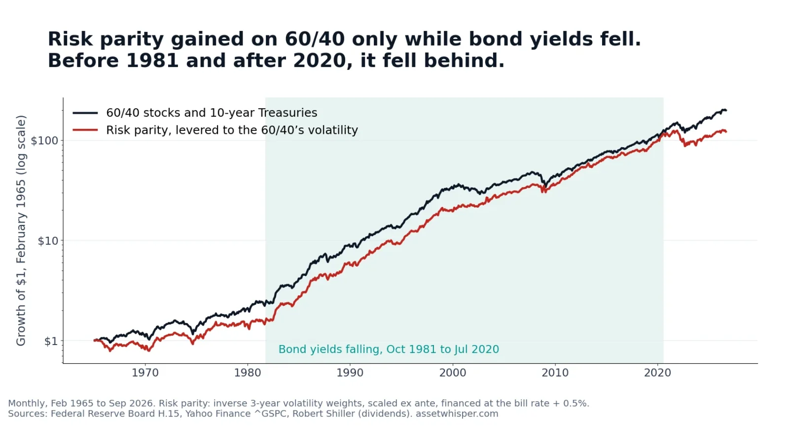
We tested both on data the papers did not use, US stocks and Treasuries from 1965 to September 2026 for risk parity and the years after publication for volatility management, with rules an investor could have followed at the time. Risk parity trailed 60/40 over the full period, with a Sharpe ratio of 0.35 against 0.45, and lost 28% in 2022 against 17%. It won only while bond yields were falling, from 1981 to 2020. Volatility management did what it is best at, cutting the loss from the October 2007 peak to February 2009 from 50% to 30%, but its Sharpe-ratio gain did not survive outside the decades that produced it.
The short answer, in one table
US stocks (the S&P 500 with dividends) and 10-year Treasuries, monthly rebalancing, February 1965 to September 2026. The Sharpe ratio is return over Treasury bills per unit of volatility. All strategies pay 5 basis points per unit of turnover; the levered version also pays the bill rate plus 0.5% on borrowed money.
| 1965–2026 | Return a year | Volatility | Sharpe | Worst fall |
|---|---|---|---|---|
| 60/40 | 8.96% | 9.89% | 0.45 | −29.4% |
| Risk parity, unlevered | 7.71% | 7.72% | 0.40 | −18.7% |
| Risk parity, levered with hindsight | 8.45% | 9.89% | 0.40 | −23.8% |
| Risk parity, levered in real time | 8.10% | 10.46% | 0.35 | −30.3% |
| Stocks alone | 10.51% | 15.04% | 0.43 | −51.0% |
| 10-year Treasuries alone | 5.82% | 8.03% | 0.17 | −26.2% |
“Levered with hindsight” uses one leverage factor (1.28) chosen after the fact so that its volatility matches the 60/40’s over the whole period, which is how the 2012 paper built its main portfolio. “Levered in real time” sets the leverage each month from the previous three years only. Every version of risk parity had a lower Sharpe ratio than 60/40 in this sample, and the version an investor could actually have run had the lowest.
What risk parity is, and the case for it
A 60/40 portfolio splits money 60/40, but not risk. Stocks were 1.9 times as volatile as 10-year Treasuries in our data, so they accounted for 86% of the 60/40’s variance. Risk parity weights each asset by the inverse of its volatility, so each contributes a similar amount of risk. On its own that means mostly bonds (our unlevered version averaged 34% stocks) and a lower return, so risk parity funds borrow to scale the whole portfolio up to the risk level of a 60/40.
Clifford Asness, Andrea Frazzini and Lasse Pedersen gave this a theory in the Financial Analysts Journal in 2012. Many investors cannot or will not borrow, so to get more return they buy more stocks. That bids up risky assets and leaves safer ones with higher returns per unit of risk, which an investor willing to use leverage can collect. In their US data from 1926 to 2010, bonds had a Sharpe ratio of 0.47 and stocks 0.35, and the levered risk-parity portfolio earned 0.53 against 0.40 for 60/40. The authors were explicit about one limit: their simulation “does not reflect any adjustment of the returns for the costs of leverage.”
Why our test disagrees: risk parity is a bet on bonds
The theory needs safer assets to earn more per unit of risk. In our sample they did not. From 1965 to 1999, 10-year Treasuries had a Sharpe ratio of 0.12 and stocks 0.40; from 2000 to 2026, bonds 0.25 and stocks 0.47. A strategy that overweights the asset with the worse risk-adjusted return, and borrows to do it, should lag, and it did. The result depends almost entirely on which decades the backtest covers:
| Period | 60/40 | Risk parity | 60/40 Sharpe | RP Sharpe |
|---|---|---|---|---|
| Feb 1965 – Sep 1981, yields rising | 4.87% | 2.22% | −0.15 | −0.36 |
| Oct 1981 – Jul 2020, yields falling | 10.87% | 11.92% | 0.72 | 0.82 |
| Aug 2020 – Sep 2026, yields rising | 8.31% | 1.02% | 0.50 | −0.11 |
Returns a year; risk parity is the real-time levered version. The breakpoints are the 10-year yield’s peak (15.32% monthly average, September 1981) and its low (0.62%, July 2020). In the four decades when yields fell, risk parity beat 60/40 by about a point a year; that window covers the last 29 years of the 2012 paper’s sample. In the sixteen years before and the six years after, it fell well behind.
Two checks on that conclusion. First, the bond: the 2012 paper used the value-weighted Treasury index, with an average duration of 5.6 years, and its authors note that their results “would be weaker with longer-term bonds”. So we reran everything with a 5-year Treasury, whose duration is shorter still. The ranking did not change: a Sharpe ratio of 0.34 for real-time risk parity against 0.45 for 60/40, with the same pattern by period. Second, the date sensitivity is a known result. Robert Anderson, Stephen Bianchi and Lisa Goldberg found in the same journal in 2012 that “even over periods lasting decades, the start and end dates of a backtest can have a material effect on results”, and that transaction costs can reverse the ranking when leverage is used.
The correlation between stocks and bonds matters too, and it moved: +0.29 in monthly returns from 1965 to 1999, −0.34 from 2000 to 2020, and +0.50 from 2021 to 2026. When bonds fall with stocks, a portfolio that holds twice the bonds offers less protection, not more, the regime shift we covered in Is 60/40 still alive?
2022: what leverage on bonds does in a bond bear market
2022 is the clearest single test. Stocks fell 18.2% and 10-year Treasuries 16.4%. A 60/40 lost 17.1%. Real-time risk parity lost 28.0%, because it held far more bonds than a 60/40 and had borrowed to hold them. With the 5-year bond the gap was wider still: −32.0% against −14.4%.
- Depth: from December 2021 to September 2022 risk parity fell 30.3%, its worst fall in 61 years. The 60/40’s worst fall in the same window was 20.9%.
- Time: risk parity did not regain its December 2021 level until May 2026. At the end of September 2026 it was 2.5% below it, while the 60/40 was 32.2% above.
- Where it stands: in September 2026 the real-time version held 43% in stocks and 77% in bonds, 1.2 times its capital and nearly twice the 60/40’s bond weight.
It also works the other way. In 2008 stocks fell 37.0%, bonds rose 20.5%, and risk parity lost only 2.9% against 17.4% for 60/40. That is what the strategy is built for: a crash in which bonds rally. It is the inflation-driven sell-off in both, as in the 1970s and 2022, that it handles worst.
Costs add up as well. Each 0.5 point of financing spread on the borrowed portion cost about 0.2 points a year of return (8.32% with no spread, 8.10% at 0.5%, 7.87% at 1%), before management fees, which our test leaves out.
Volatility targeting: what the paper found, and what came after
Alan Moreira and Tyler Muir took a different route to the same goal. Their rule scales exposure to the stock market by the inverse of the previous month’s realized variance: when the market has just been volatile, hold less; when it has been calm, hold more. Volatility clusters, so a volatile month tends to be followed by another, but it does not reliably predict higher returns. On the US market from 1926 to 2015, they reported an alpha of 4.9% a year and “an overall 25% increase in the buy-and-hold Sharpe ratio.”
We replicated the rule on Kenneth French’s daily market data. Over the paper’s own period we get the same answer: a Sharpe ratio of 0.51 for the managed portfolio against 0.42 for the market, an increase of 23%. Broken into periods, and after the paper appeared, the picture changes.
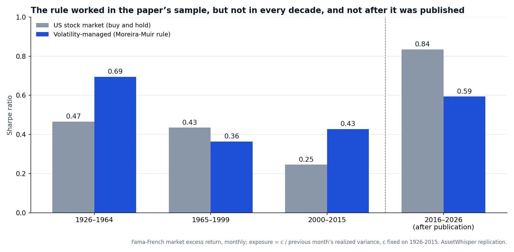
The rule helped in 1926–1964 and 2000–2015, hurt from 1965 to 1999, and from January 2016 to August 2026 it cut the market’s Sharpe ratio from 0.84 to 0.59, a 29% fall. A larger study points the same way. Scott Cederburg, Michael O’Doherty, Feifei Wang and Xuemin Yan tested 103 equity strategies in the Journal of Financial Economics in 2020: the volatility-managed version had the higher Sharpe ratio in 53 cases and the lower in 50, only eight differences were statistically significant, and for the market itself a version implementable in real time earned 0.42 against 0.46 for simply holding it.
The simpler version: a volatility target
Most funds use a plainer rule: aim for a fixed volatility, here 15% a year, close to the S&P 500’s long-run level, by setting next month’s exposure to 15% divided by last month’s realized volatility, with a cap of 1.5 times capital. February 1965 to September 2026:
| S&P 500, 1965–2026 | Return a year | Volatility | Sharpe | Worst fall |
|---|---|---|---|---|
| Buy and hold | 10.51% | 15.04% | 0.43 | −51.0% |
| 15% volatility target, cap 1.5× | 10.79% | 15.50% | 0.44 | −40.4% |
| Fixed 116% in stocks (same average exposure) | 11.22% | 17.42% | 0.43 | −56.7% |
| Moreira–Muir rule, constant set with hindsight | 9.57% | 15.06% | 0.38 | −48.9% |
The target mostly levered up: calm months are the norm, so its average exposure was 116% of capital, and it sat at the 1.5× cap in 30% of months. Against a fixed 116% in stocks it returned 0.4 points a year less, with much less volatility and a worst fall 16 points shallower. Its Sharpe ratio edged buy-and-hold by 0.01 over the whole period, but that hides a split: 0.37 against 0.40 from 1965 to 1999, 0.57 against 0.47 from 2000 onwards. After the Moreira–Muir paper appeared, from July 2016 to September 2026, the two had the same Sharpe ratio (0.86), and the target returned 15.00% a year against 15.30%.
What it did consistently was soften slow crises:
- October 2007 to February 2009: −29.9% against −50.2% for the index.
- January to September 2022: −18.3% against −23.9%.
- September to December 1987: −17.5% against −24.2%. The rule went into October 84% invested and took most of the crash; the rest of the gap came from holding only 16% in November.
- February to March 2020: −17.2% against −19.6%. The rule entered February 26% levered after a calm January; a crash that comes out of calm is the one it cannot see.
That is the same trade-off as the 10-month moving-average rule: a shallower worst case in slow bear markets, paid for with trading (2.4 times capital a year here) and, for a taxable investor, realised gains.
What the record supports, and what it does not
- Supported: risk parity outperformed 60/40 when bond yields fell, as from 1981 to 2020, and protected well in crashes where bonds rallied, as in 2008.
- Supported: volatility targeting reduced the worst losses in slow bear markets, by 20 points in 2007–09.
- Not supported: that risk parity beats 60/40 in general. From 1965 to 2026 it did not, with either a 10-year or a 5-year bond, and it lost most in 2022.
- Not supported: that volatility management reliably raises the Sharpe ratio. Our replication of the 2017 rule lost 29% of the market’s Sharpe ratio after publication, consistent with the 2020 study of 103 strategies.
- Not tested: multi-asset risk parity with commodities, credit or inflation-linked bonds, other countries, and management fees. Real funds differ in all of these.
Both ideas are better read as risk tools than as return engines, which is also how position sizing should be read. And both rely on leverage at some point, which brings the arithmetic of volatility drag with it.
Frequently asked questions
What is risk parity?
A way of building a portfolio so that each asset contributes a similar amount of risk rather than a similar amount of money. Because bonds are less volatile than stocks, it holds more bonds, and most versions borrow to bring the total risk up to the level of a 60/40 portfolio.
Does risk parity beat a 60/40 portfolio?
It depends on the period. In the 2012 study covering 1926–2010 it did, with a Sharpe ratio of 0.53 against 0.40. In our test from 1965 to September 2026 it did not: 0.35 against 0.45 for the version an investor could have run in real time. It won from 1981 to 2020, when bond yields fell, and lost before and after.
Why did risk parity lose so much in 2022?
Because stocks and bonds fell together and risk parity holds a large, levered bond position. In our simulation it lost 28.0% in 2022 against 17.1% for 60/40, and took until May 2026 to regain its December 2021 level.
What is volatility targeting?
A rule that adjusts how much of a portfolio is invested according to recent volatility: less after volatile periods, more after calm ones, aiming at a fixed level of risk. A 15% target on the S&P 500 averaged 116% invested from 1965 to 2026, because calm months are more common.
Does volatility targeting improve returns?
Not reliably. In our test it matched buy-and-hold on return per unit of risk overall and after 2016, but it cut the worst fall from 51.0% to 40.4% and the 2007–09 loss from 50.2% to 29.9%. The stronger variance-scaling rule from the 2017 paper lowered the Sharpe ratio after publication.
Should I use leverage to build a risk parity portfolio?
This article cannot answer that for any individual. It describes what simulated strategies did in the past under stated assumptions; leverage adds financing costs and the risk of losses larger than an unlevered portfolio’s. AssetWhisper does not publish trade signals or recommendations.
How we calculated this
- Stocks: daily S&P 500 closes (Yahoo Finance ^GSPC) plus one 252nd of Robert Shiller’s dividend yield per session. Annual returns from 1963 to 2025 match Damodaran’s S&P 500 series (correlation 1.000; 10.76% a year against 10.75%). Each asset is compounded to months on its own trading calendar, because the stock and bond markets do not close on the same holidays.
- Bonds: a constant-maturity 10-year Treasury (and, for the check, a 5-year), repriced every day from the Federal Reserve’s H.15 yields as a par bond with semiannual coupons. Annual returns from 1963 to 2025 correlate at 0.988 with Damodaran’s 10-year Treasury series, compounding at 5.88% a year against his 5.54%.
- Cash: 3-month Treasury bill, H.15, converted to a bond-equivalent yield.
- Risk parity: at each month-end, weights proportional to the inverse of each asset’s volatility over the previous 36 months of monthly excess returns, as in Asness, Frazzini and Pedersen (2012). Unlevered: weights sum to one. Levered with hindsight: one constant (1.28) that matches the 60/40’s full-period volatility. Levered in real time: leverage set each month so the portfolio’s volatility over the previous 36 months, at current weights, matches the 60/40’s over the same window, capped at 4× (the cap bound in 9 months, March to November 1965, when bond volatility over the previous three years had been unusually low).
- Volatility target: exposure for each month = 15% divided by the previous month’s realized volatility of daily returns, annualised, capped at 1.5×. Borrowing at the bill rate plus 0.5%.
- Moreira–Muir replication: Fama–French daily market excess returns, July 1926 to August 2026; monthly exposure = c divided by the previous month’s realized variance, with c set so the managed portfolio has the market’s volatility over 1926–2015 and then held fixed.
- Costs and limits: 5 basis points per unit of turnover; no taxes or fund fees. Sample starts in February 1965 because daily 10-year yields begin in 1962 and the rules need three years of history. One country, two assets. The script that prints every figure is kept with this article’s working files.
Sources
- Clifford S. Asness, Andrea Frazzini and Lasse H. Pedersen, “Leverage Aversion and Risk Parity”, Financial Analysts Journal, 68(1), 2012, pp. 47–59. Table 2, Panel A for the 1926–2010 figures.
- Alan Moreira and Tyler Muir, “Volatility-Managed Portfolios”, Journal of Finance, 72(4), 2017. Figures quoted from the NBER working paper 22208 (April 2016, revised June 2016).
- Scott Cederburg, Michael S. O’Doherty, Feifei Wang and Xuemin (Sterling) Yan, “On the Performance of Volatility-Managed Portfolios”, Journal of Financial Economics, 138, 2020, pp. 95–117.
- Robert M. Anderson, Stephen W. Bianchi and Lisa R. Goldberg, “Will My Risk Parity Strategy Outperform?”, Financial Analysts Journal, 68(6), 2012.
- Board of Governors of the Federal Reserve System, H.15 Selected Interest Rates: 10-year and 5-year constant-maturity yields, 3-month bill, daily from 1962.
- Kenneth R. French, Data Library: Fama–French factors, daily, to August 2026.
- Robert J. Shiller, U.S. stock market data (dividends); Yahoo Finance, ^GSPC; Aswath Damodaran, historical returns (bond validation).
Related reading
- Is 60/40 still alive? — the stock–bond correlation regime that decides how both portfolios behave.
- Volatility drag — what leverage does to compounding.
- The 10-month moving average on the S&P 500 — another rule that trades return for a shallower worst case.
- How often to rebalance — the cost side of any rule that trades monthly.
This article is general information, not personalised investment advice. It does not take into account the financial situation, objectives, tax position or risk tolerance of any individual reader, and the same text is distributed to all readers. Simulated results describe the past under stated assumptions and are not forecasts. Leveraged strategies can lose more than unlevered ones, and borrowing costs and fees reduce returns. Capital is at risk.