Do High-Dividend Stocks Beat the Market? 99 Years of US Data, Before and After Value
Key takeaway
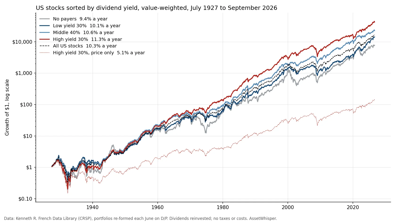
From July 1927 to September 2026 the highest-yielding 30% of US stocks compounded at 11.34% a year against 10.26% for the market. Most of that edge is the value premium: after size and value, 0.21 points a year are left. The top 10% by yield did worse than the next two groups, with more risk.
Dividend investing is usually argued from anecdote: a company that has raised its payout for 50 years, a retiree living off the cheques. We wanted the other kind of answer. Every June since 1927, Kenneth French’s data library sorts the US stocks in the CRSP database by dividend yield, the dividends of the past year divided by the share price, and records what each group returned over the following twelve months. The database covers NYSE stocks from the start, adds AMEX in 1962 and Nasdaq in 1972, and has no survivorship bias. That gives 99 years and 3 months of returns for stocks that paid nothing, paid little, paid an average amount or paid a lot.
The highest-yielding 30% compounded at 11.34% a year against 10.26% for the whole market, from July 1927 to September 2026. Most of that edge is the value effect under another name: once the portfolio’s tilt toward cheap stocks is accounted for, what is left is 0.21 points a year, statistically indistinguishable from zero. The very highest yielders did worse than the next two groups down, with more volatility, and since 2010 the high-yield group trailed the market.
The short answer, in one table
Value-weighted portfolios, re-formed each June, dividends reinvested, no taxes or trading costs. “Price only” is the same portfolio with the dividends left out, the part of the return that showed up as a higher share price. “From dividends” is the difference between the two compound rates, so “Price only” and “From dividends” add up to the total, give or take 0.01 from rounding.
| Jul 1927–Sep 2026 | Return a year | Price only | From dividends | Volatility | Sharpe |
|---|---|---|---|---|---|
| No payers | 9.44% | 8.54% | 0.91% | 28.0% | 0.34 |
| Low yield 30% | 10.12% | 7.62% | 2.50% | 19.4% | 0.43 |
| Middle 40% | 10.62% | 6.37% | 4.25% | 17.6% | 0.48 |
| High yield 30% | 11.34% | 5.07% | 6.26% | 19.6% | 0.48 |
| All US stocks | 10.26% | n/a | n/a | 18.4% | 0.45 |
A dollar put in the high-yield group in July 1927 was worth $42,566 in September 2026, against $16,290 in the whole market and $7,753 in the stocks that paid nothing. Two things in the table matter more than that ranking. The return went up with the yield, but the price return went down with it, almost in step: the high-yield group’s share prices compounded at only 5.07% a year, so a dollar in it without the dividends grew to $136. And the extra return came with no reduction in risk. The high-yield group was more volatile than the market and its worst fall, in 1929–32, was 87.9%, against 83.7% for the market.
Where the return came from: price and dividends
A dividend does not add to an investor’s wealth on the day it is paid. The share price drops by about the amount paid out, so the investor holds the same value in two pieces, part cash and part shares; our guide to the advantages of dividend investing walks through that mechanic. Merton Miller and Franco Modigliani proved in 1961 that, in a market without taxes or trading costs and for a given investment policy, how a company splits its earnings between dividends and retained earnings does not change what its shares are worth.
The table shows what that looks like over a century. The more a group paid out, the less its price grew. In the high-yield group dividends were 54% of the total return (measured in log terms, so that the shares add up over time); in the low-yield group, 24%; in the non-payers, 9%. The non-payers’ figure is not zero because some of them start paying during the year after they are sorted. The high-yield group did not turn the same companies into more money by paying them out. It was a different set of companies, cheaper ones, and that is what the next section tests.
Is it a dividend premium, or the value premium?
A high dividend yield is a low price relative to a stream of cash. So is a high book-to-market ratio, the measure Eugene Fama and Kenneth French used in 1993 to define value stocks. If the high-yield group earned more because it held cheap stocks, the extra return should disappear once its exposure to the value factor (HML, high minus low book-to-market) is accounted for. We ran that regression on monthly returns over the whole 99 years, with Newey-West standard errors, which are robust to heteroskedasticity and autocorrelation.
| 1927–2026 | Market only | + size, value | Value beta |
|---|---|---|---|
| No payers | −2.04 (t −1.9) | −2.41 (t −2.8) | 0.03 |
| Low yield 30% | −0.06 (t −0.1) | +0.55 (t 1.1) | −0.20 |
| Middle 40% | +0.84 (t 1.5) | +0.50 (t 1.0) | 0.15 |
| High yield 30% | +1.63 (t 1.7) | +0.21 (t 0.3) | 0.50 |
| High minus low | +1.68 (t 1.3) | −0.35 (t −0.3) | 0.70 |
Alphas are in percentage points a year, July 1927 to September 2026, with Newey-West t-statistics in parentheses; a t-statistic below about 2 means the alpha cannot be told apart from zero. Against the market alone, the high-yield group earned 1.63 points a year more than its market risk explained, and even that was not significant. Add size and value and it falls to 0.21 points. The high-yield group’s value beta of 0.50 is large: it behaved like a portfolio with half its money in a long-short value strategy. The high-minus-low spread loads 0.70 on value and has nothing left.
Even the raw gap is weaker than it looks. The high-yield group beat the low-yield group by 1.05 points a year on average, with a t-statistic of 0.7 over 99 years: the difference is there in the compound returns, and statistically it is noise. The value factor itself averaged 4.13 points a year over the same months.
Two other standard models can be checked. Fama and French’s five-factor model of 2015 can only be run from July 1963, when its data begin, so to compare like with like all three are run on that window:
| 1963–2026 | + size, value | + momentum | Five-factor |
|---|---|---|---|
| No payers | −0.10 (t −0.1) | −0.25 (t −0.4) | +1.35 (t 1.7) |
| High yield 30% | +0.04 (t 0.1) | +0.96 (t 1.4) | −1.10 (t −1.6) |
| Top 10% by yield | −0.31 (t −0.2) | +1.10 (t 0.7) | −0.98 (t −0.8) |
| High minus low | −0.58 (t −0.5) | +0.74 (t 0.6) | −1.11 (t −1.0) |
Adding momentum, the tendency of recent winners to keep winning that Mark Carhart added to the model in 1997, raises the high-yield group’s alpha to 0.96 points, because high yielders tend to be recent losers and the model credits them for having earned more than momentum predicts. Adding profitability and investment instead turns it to −1.10 points: the profitable, slow-investing companies that pay dividends explain the rest. None of the three is significant. Over the whole sample from 1927 the momentum model does give the high-yield group an alpha of 1.65 points with a t-statistic of 2.3, but that comes from the years before 1963, when it was 2.90 points; since then it has been 0.96 with a t-statistic of 1.4. A premium that depends on which model and which decades are used is not a robust one. What every version agrees on is the value loading: the high-yield group was always a value portfolio. The same goes for the non-payers: their significant shortfall over the full sample (−2.41 points) also comes from before 1963, and since then the three-factor alpha has been −0.10.
When high yield won, and when it did not
A 99-year average hides long stretches in which the ranking reversed.
| Return a year | No payers | Low 30% | Mid 40% | High 30% | Market |
|---|---|---|---|---|---|
| 1927–1962 | 7.67% | 8.38% | 9.98% | 9.87% | 9.02% |
| 1963–1999 | 12.75% | 12.66% | 12.07% | 13.56% | 12.79% |
| 2000–Sep 2026 | 7.33% | 8.97% | 9.50% | 10.26% | 8.48% |
| 2010–Sep 2026 | 14.29% | 15.27% | 12.98% | 13.23% | 14.15% |
All of the high-yield group’s lead after 2000 came in three years. From 2000 to 2002, as the technology bubble burst, it gained 7.9% a year while the non-payers lost 27.5% a year and the market lost 14.8%. From January 2003 to September 2026 it compounded at 10.6% a year against 11.8% for the market. From 2010 to 2026 the high-minus-low spread averaged −2.30 points a year and the value factor −0.67: the two moved together again.
Single years show the same pattern. In 2020 the high-yield group lost 2.7% while the market gained 24.1%. In 2022 it gained 7.7% while the market lost 19.9%. A dividend tilt is a bet on which kind of company the market will favour, and in some years it is a large one.
The top 10%: where a high yield turns into a warning
Yield is the dividend divided by the price, and the price moves every day while the dividend changes once or twice a year. So a stock can reach the very top of a yield ranking because its price has fallen, and a falling price can come before a cut in the payment. These data do not record dividend cuts, so they cannot say how much of the result that explains. What they do show is that the top decile was the most extreme value portfolio of all, and how it did:
| Jul 1927–Sep 2026 | Return a year | Volatility | Sharpe | Value beta | 2008 |
|---|---|---|---|---|---|
| 8th decile | 11.8% | 19.3% | 0.50 | 0.40 | −28.5% |
| 9th decile | 11.3% | 20.1% | 0.47 | 0.47 | −26.6% |
| Top decile | 10.7% | 22.6% | 0.41 | 0.75 | −47.9% |
| All US stocks | 10.3% | 18.4% | 0.45 | n/a | −36.7% |
The top decile earned less than the 8th and 9th, with more volatility, a lower Sharpe ratio than the market and the strongest value loading of any group. After size and value, its alpha was −0.93 points a year (t −0.9). In calendar 2008 it fell 47.9%, against 36.7% for the market and less than 30% for the two deciles below it; from its 2007 peak to its 2009 low it lost 73.4%, against 50.3% for the market. It was not the worst decile that year: the lowest-yielding 10% of payers fell 54.5%. Since 2000 the top decile has done better, at 11.3% a year, the highest of the ten: the warning shows up in the risk numbers more consistently than in the returns.
The announcement of a cut moves prices on its own. Roni Michaely, Richard Thaler and Kent Womack found that share prices react more to dividend omissions than to initiations, and keep drifting in the same direction for a year afterwards, with the drift after omissions stronger. A yield screen is likely to hold more of the companies exposed to that announcement, though this study measures omissions, not the make-up of yield deciles.
The homemade dividend, with US taxes
Miller and Modigliani’s argument has a practical form. An investor who wants $4,000 a year from a $100,000 portfolio can get it from a dividend or by selling shares. Before taxes the two are the same. After taxes, they differ mainly in when the tax is paid:
| $100,000, cost $60 a share | 4% dividend | Sell 40 shares |
|---|---|---|
| Cash received | $4,000 | $4,000 |
| Shares afterwards | 1,000 at $96 | 960 at $100 |
| Tax now, at 15% | $600 | $240 |
| Gain left in the shares | $36,000 | $38,400 |
| Tax on it if sold later | $5,400 | $5,760 |
| Total tax | $6,000 | $6,000 |
In the US, qualified dividends are taxed at the same rates as long-term capital gains, 0%, 15% or 20% depending on taxable income, plus the 3.8% net investment income tax on investment income above $200,000 of modified adjusted gross income for a single filer and $250,000 for a married couple filing jointly, according to the IRS. A dividend counts as qualified if, among other conditions, the shares were held for more than 60 days of the 121-day period that begins 60 days before the ex-dividend date; otherwise it is taxed as ordinary income. The dividend is taxed in full, while the sale is taxed only on the gain: in the example, $60 of every $100 sold is a return of the investor’s own money. That is why the seller pays $240 now instead of $600. But the seller is left with $2,400 more of unrealised gain in the remaining shares, and if both investors later sell everything at the same rate, the total tax is the same. The dividend brings the tax forward; it does not make it larger. Paying later is worth something, because the money not yet paid in tax stays invested. The difference becomes permanent mainly when the shares are never sold: inherited shares generally take a new cost basis equal to their market value at the owner’s death. Qualified dividends are also taxed at 0% in the 0% band, so that band changes nothing on its own; part of the tax is saved for good only if the dividend was taxed at 15% and the later sale falls in the 0% band, for example after income drops in retirement. The dividend is also taxed whether or not the investor needed the cash that year, and reinvested dividends are taxed the same way. Inside an IRA or a 401(k), neither the dividend nor the sale is taxed when it happens; withdrawals follow the account’s own rules.
This is the general federal framework, not advice for any reader’s situation. State taxes, foreign withholding on dividends from non-US companies and the investor’s bracket all change the numbers; our study of the 4% rule deals with how much can be withdrawn, whichever way the cash is raised.
Why investors prefer dividends anyway
If a dividend is a withdrawal that is taxed sooner, why is there so much demand for it? Hersh Shefrin and Meir Statman proposed in 1984 that dividends help investors control their own spending: a rule of “spend the income, never touch the capital” is easier to keep than a plan to sell a little every year, even when the two are equivalent.
Samuel Hartzmark and David Solomon documented the cost of thinking that way. Investors, mutual funds and institutions, they found, trade as if dividends and price changes were separate things, not fully appreciating that a dividend lowers the price. They rarely reinvest dividends, they treat them as a separate and stable stream of income, and analysts forecast prices for dividend payers that are too optimistic because they do not account for the drop the dividend causes. They call it the free dividends fallacy. Demand for dividends rises when interest rates are low and markets have done badly, and in their sample it was followed by lower returns for dividend payers. They also found that the disposition effect, one of the biases our review of behavioural biases puts a number on, is driven by price changes rather than total returns.
There is also less to choose from than there used to be. In June 1978, 32% of the stocks in French’s sample paid no dividend; by June 1999 it was 69%, by June 2000, 70%, and in June 2026, 61%. Fama and French, counting only non-financial, non-utility firms, found that the share of payers fell from 66.5% in 1978 to 20.8% in 1999, and that only part of the fall came from the arrival of small, unprofitable listings: companies with the same characteristics had become less likely to pay. Gustavo Grullon and Roni Michaely showed in 2002 that companies had gradually substituted share buybacks for dividends, paying with buybacks cash that would otherwise have gone to raise the dividend. A yield screen does not see that cash.
What the evidence supports, and what it does not
- It supports: stocks with higher dividend yields earned more than low-yield and non-paying stocks over 99 years of US data, with similar risk, and most of the difference was compounded dividends rather than price gains.
- It supports: the difference is mostly the value premium. With size and value in the model, no dividend premium is left. On the same 1963–2026 window, adding momentum gives an alpha of 0.96 points and adding profitability and investment one of −1.10, neither significant: a result that depends on the model is not a robust premium.
- It does not support: chasing the highest yields. The top decile earned less than the two below it, was more volatile than the market and fell 47.9% in 2008, against 36.7% for the market.
- It does not support: treating dividends as extra return. Before taxes a dividend is a withdrawal; after taxes, for an investor in a taxable US account, it brings the tax bill forward compared with selling shares.
- It cannot say: whether the next 20 years will look like 1927–1999 or like 2010–2026. A value tilt has gone a decade and more without paying.
The comparison in our look at index funds against active managers is relevant here: a dividend strategy is a factor tilt with costs, and the evidence for the tilt is the evidence for value. How small differences in return compound over decades is set out in our compound interest calculation, and why a portfolio with the same average return but more volatility ends with less in our explanation of volatility drag. To try other return and withdrawal assumptions, use the investment calculator.
Frequently asked questions
Do high-dividend stocks outperform the market?
In US data from July 1927 to September 2026, the highest-yielding 30% of stocks compounded at 11.34% a year against 10.26% for the market. The gap is not statistically significant, and after adjusting for the value factor it shrinks to 0.21 points a year. It also reversed for long periods, including 2010 to 2026.
Is the dividend premium just the value premium?
Mostly. A high yield is a low price relative to cash paid out, which is what value stocks are. In a regression on market, size and value, the high-yield group’s alpha was 0.21 points a year and its value beta 0.50. From 1963, adding momentum gives an alpha of 0.96 points and using profitability and investment instead one of −1.10; neither is significant.
Why did the highest-yielding stocks do worse than the next groups down?
The data do not say why. The top 10% by yield was the most extreme value portfolio of all (value beta 0.75), and a very high yield often reflects a falling price that can come before a dividend cut. It earned 10.7% a year against 11.3% for the 9th decile and 11.8% for the 8th, with 22.6% volatility, and fell 47.9% in 2008.
Are dividends taxed more than selling shares in the US?
Qualified dividends are taxed at the same 0%, 15% or 20% rates as long-term capital gains, but on the whole amount, while a sale is taxed only on the gain above its cost. Much of the difference is timing: the gain left in unsold shares is taxed when they are sold. Dividends are taxed in the year paid, even if reinvested. Inside an IRA or a 401(k), neither is taxed when it happens.
What is the free dividends fallacy?
The name Samuel Hartzmark and David Solomon gave, in “The Dividend Disconnect” (Journal of Finance, 2019), to investors treating dividends as income on top of the share price, rather than as cash taken out of it. They found it in the trading of individuals, mutual funds and institutions, and in analysts’ price forecasts.
How we calculated this
- Portfolios: Kenneth R. French Data Library, “Portfolios Formed on Dividend Yield”, built from the CRSP database of September 2026. All NYSE, AMEX and Nasdaq stocks in CRSP with a June market value and at least 7 monthly returns in the prior year are sorted at the end of each June on dividends paid from July to June per dollar of June market value, using NYSE breakpoints. Non-payers form their own group. In July 1927 the portfolios hold 547 stocks; they pass 1,000 in 1951. Because of that requirement, AMEX stocks enter the portfolios from July 1963 and Nasdaq stocks from July 1973. Value-weighted monthly returns, July 1927 to September 2026 (1,191 months).
- Price only: the same library’s “Portfolios Formed on Dividend Yield [ex. Dividends]”. “From dividends” is the total compound rate minus the price-only compound rate. The dividend share of the return is the difference in summed log returns, divided by the summed log total return.
- Market and factors: French’s Fama-French three-factor file, momentum factor (July 1927 on) and five-factor file (July 1963 on). The market is all CRSP firms, value-weighted, and includes recent listings that the dividend-yield portfolios exclude, so the two universes differ slightly. For the July 1963 to September 2026 comparison, all three models use the market, size and value factors from the five-factor file, so the models are nested; with the three-factor file, the non-payers’ alphas would be −0.21 and −0.37 instead of −0.10 and −0.25, and the other figures in the table change by 0.03 points or less. The risk-free rate is the one-month Treasury bill in those files.
- Statistics: returns a year are compound annual growth rates. Volatility = standard deviation of monthly returns × √12. Sharpe ratio = annualised mean monthly excess return over its standard deviation. Alphas are regression intercepts on monthly excess returns, times 12, with Newey-West standard errors at 6 lags (12 lags changes no conclusion); the t-statistic of the raw spread is from a regression on a constant with the same errors. Worst falls are on month-end values.
- Tax example: illustrative, federal rates only, assuming qualified dividends and long-term gains taxed at 15%, a cost basis of $60 a share and the same rate for the later sale; the equal totals hold at any later price, because the two portfolios are worth the same and differ only by $2,400 of unrealised gain.
- Limits: US stocks only; no taxes, trading costs or fund fees; the portfolios are research portfolios, not funds anyone could have bought before index funds existed; one historical path. Past returns are not a forecast. The script that prints every figure and draws the chart is kept with this article’s working files.
Sources
- Merton H. Miller and Franco Modigliani, “Dividend Policy, Growth, and the Valuation of Shares”, Journal of Business, 34(4), 1961, pp. 411–433.
- Eugene F. Fama and Kenneth R. French, “Common Risk Factors in the Returns on Stocks and Bonds”, Journal of Financial Economics, 33(1), 1993, pp. 3–56.
- Eugene F. Fama and Kenneth R. French, “A Five-Factor Asset Pricing Model”, Journal of Financial Economics, 116(1), 2015, pp. 1–22.
- Eugene F. Fama and Kenneth R. French, “Disappearing Dividends: Changing Firm Characteristics or Lower Propensity to Pay?”, Journal of Financial Economics, 60(1), 2001, pp. 3–43.
- Gustavo Grullon and Roni Michaely, “Dividends, Share Repurchases, and the Substitution Hypothesis”, Journal of Finance, 57(4), 2002, pp. 1649–1684.
- Mark M. Carhart, “On Persistence in Mutual Fund Performance”, Journal of Finance, 52(1), 1997, pp. 57–82.
- Samuel M. Hartzmark and David H. Solomon, “The Dividend Disconnect”, Journal of Finance, 74(5), 2019, pp. 2153–2199.
- Hersh M. Shefrin and Meir Statman, “Explaining Investor Preference for Cash Dividends”, Journal of Financial Economics, 13(2), 1984, pp. 253–282.
- Roni Michaely, Richard H. Thaler and Kent L. Womack, “Price Reactions to Dividend Initiations and Omissions: Overreaction or Drift?”, Journal of Finance, 50(2), 1995, pp. 573–608.
- Whitney K. Newey and Kenneth D. West, “A Simple, Positive Semi-Definite, Heteroskedasticity and Autocorrelation Consistent Covariance Matrix”, Econometrica, 55(3), 1987, pp. 703–708.
- Internal Revenue Service, Topic no. 404, Dividends and other corporate distributions; Topic no. 409, Capital gains and losses; Topic no. 559, Net investment income tax; Publication 550, Investment Income and Expenses (holding period for qualified dividends, reinvested dividends); Publication 551, Basis of Assets (inherited property).
- Data: Kenneth R. French, Data Library (Portfolios Formed on Dividend Yield, with and without dividends; Fama/French 3 Factors; 5 Factors (2×3); Momentum Factor), CRSP database of September 2026. Retrieved 27 October 2026.
Related reading
- Dividend investing: the advantages, and the arithmetic most guides skip — what a dividend does to your money, buybacks and how to read a dividend fund.
- How to identify undervalued assets — the value side of the same question.
- Bear markets: depth, duration and recovery — the falls behind the worst-year numbers.
This article is general information, not personalised investment or tax advice. It does not take into account the financial situation, objectives, tax position or risk tolerance of any individual reader, and the same text is distributed to all readers. Historical and simulated results describe the past under stated assumptions and are not forecasts. Taxes, trading costs and fund fees reduce returns. Capital is at risk.