The 10-Month Moving Average on the S&P 500: What 92 Years of Data Say About Trend Following
Key takeaway
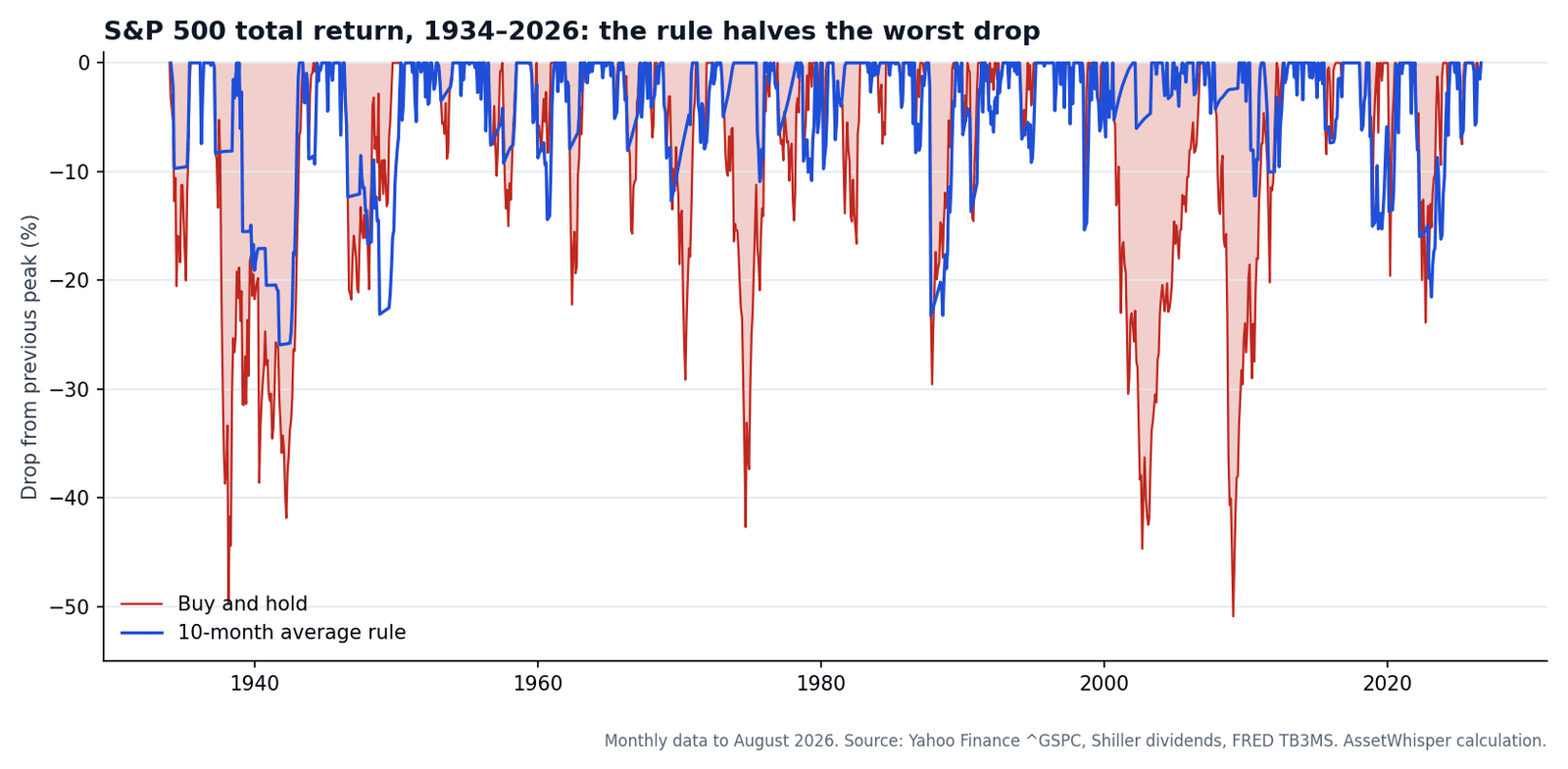
A 10-month moving-average rule on the S&P 500 returned 10.3% a year since 1934 against 11.2% for buy-and-hold, but its worst fall was 26% instead of 51%. It beat holding in only 21 of 92 years, and three-quarters of its exits were followed by a re-entry at a higher price.
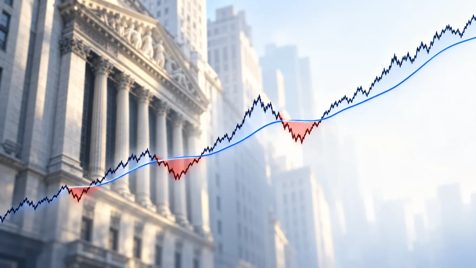
The most repeated rule in technical analysis fits in one sentence: hold stocks while the market is above its moving average, and hold cash when it is below. We tested it on the S&P 500 over 92 years, from January 1934 to August 2026, using the monthly version popularised by Mebane Faber in 2007, a 10-month simple moving average, which is close to the 200-day average traders quote (200 trading days is about 9.5 months).
The result is not the one the rule’s fans or its critics usually claim. The rule did not beat buy-and-hold on return: 10.3% a year against 11.2%. What it did was cut the worst peak-to-trough loss from 51% to 26% and avoid almost all of the damage in the long bear markets of 1937, 1973–74, 2000–02 and 2007–09. It paid for that by lagging in most calendar years and by trading about one and a half times a year, and three-quarters of its exits were followed by a re-entry at a higher price.
The short answer, in one table
The rule: at each month-end, if the S&P 500 closed above the simple average of its last 10 month-end closes, hold the index (with dividends) for the next month; otherwise hold 3-month Treasury bills. The signal is read at the close and acted on in the following month, so nothing in the test uses information from the future.
| Jan 1934 – Aug 2026 | Buy and hold | 10-month rule | Treasury bills |
|---|---|---|---|
| Return per year | 11.19% | 10.32% | 3.47% |
| Volatility (annualised) | 15.65% | 10.83% | 0.89% |
| Worst peak-to-trough fall (monthly) | −50.9% | −25.9% | none |
| Return per unit of risk (Sharpe, over bills) | 0.53 | 0.65 | n/a |
| Share of months in stocks | 100% | 69.4% | 0% |
| 1 dollar in January 1934 became | $18,500 | $8,930 | $23.51 |
The rule gave up 0.87 points a year, which compounded over nearly a century leaves less than half the final wealth. In exchange it ran with about two-thirds of the volatility and half the worst loss. Whether that is a good trade depends on whether a 51% fall would have made the holder sell at the bottom, a question closer to the behaviour costs we measured in six behavioural biases. The data here cannot answer it.
Is it the timing, or just less stock?
A fair objection: the rule was in stocks 69% of the time, so some of its lower risk is simply lower exposure. We checked by holding a fixed 69.4% in stocks and 30.6% in bills, rebalanced monthly, the same average exposure and almost the same volatility.
| Same average exposure | Return per year | Volatility | Worst fall | Sharpe |
|---|---|---|---|---|
| Fixed 69.4% stocks / 30.6% bills | 8.96% | 10.84% | −38.0% | 0.53 |
| 10-month rule (69.4% of months in stocks) | 10.32% | 10.83% | −25.9% | 0.65 |
At identical volatility, the rule earned 1.4 points a year more than the fixed mix and had a worst fall 12 points shallower. A fixed mix has the same Sharpe ratio as buy-and-hold (0.53), as it should, because it only scales risk. The rule’s 0.65 is the part that comes from timing, not from owning less. So the fair summary is two statements that are both true: it lost to full buy-and-hold on return, and it beat a portfolio with the same amount of risk.
What it did in each bear market
The edge came almost entirely from the long, grinding declines, which is what a trend rule is built for. We measured total return over each window, for both strategies. The bear markets themselves are tabulated in Bear Markets Since 1950.
| Window (month returns) | Buy and hold | 10-month rule | Months in stocks |
|---|---|---|---|
| Mar 1937 – Mar 1938 | −49.6% | −8.1% | 15% |
| Jan 1973 – Sep 1974 | −42.7% | +7.0% | 10% |
| Sep – Dec 1987 | −24.2% | −22.5% | 50% |
| Aug 2000 – Sep 2002 | −41.3% | +0.7% | 12% |
| Oct 2007 – Feb 2009 | −50.1% | −0.8% | 12% |
| Jan – Mar 2020 | −19.6% | −8.2% | 67% |
| Dec 2021 – Sep 2022 | −20.5% | −11.6% | 40% |
The pattern is clear: when a decline takes months to unfold, the index slips under its 10-month average early and the rule steps aside. When it is fast, the rule has no time. The October 1987 crash is the clearest miss: the September close was still above the average, so the rule was fully invested and lost almost as much as the index. In 2020 it was out only for March. (The sample starts in 1934, so the 1929–1932 collapse is not in it.)
What it costs: the long stretches of lagging
The same feature that protects in a bear market costs in a bull market, because the rule is in cash during every false alarm and during the early part of every recovery.
- Calendar years: the rule beat buy-and-hold in only 21 of 92 years (1934–2025), and trailed it by 10 points or more in 12 of them. The worst relative years were 1975 (21.6 points behind), 2019 (20.6), 1991 (17.3) and 2023 (16.5), all strong rebounds after a decline.
- Ten-year windows: over 991 rolling ten-year periods the rule was ahead in 41%, with a median of 1.1 points a year behind. Its best ten years ended in February 2009 (10.4 points a year ahead), its worst in July 1994 (7.1 behind).
- The last bull market: from April 2009 to August 2026 buy-and-hold returned 15.95% a year against 9.94% for the rule, a gap of six points a year, while the rule’s worst fall (−21.5%) was only two and a half points better than the index’s (−23.9%).
| Period | Buy and hold: return / worst fall | 10-month rule: return / worst fall |
|---|---|---|
| 1934–1949 | 8.95% / −49.6% | 7.41% / −25.9% |
| 1950–1974 | 9.98% / −42.7% | 11.73% / −14.4% |
| 1975–1999 | 17.11% / −29.5% | 12.68% / −23.2% |
| 2000–Aug 2026 | 8.31% / −50.9% | 8.59% / −21.5% |
| Apr 2009–Aug 2026 | 15.95% / −23.9% | 9.94% / −21.5% |
Taken period by period, the rule won on return in two of the four non-overlapping blocks (1950–74 and 2000–26) and lost in the other two. Both blocks it won contain long bear markets (1973–74, then 2000–02 and 2007–09). Where it lost most, 1975–1999, the market had a fast crash in 1987 and a mostly uninterrupted climb.
Whipsaws: the price of being early
The rule left the market and came back 70 times, 141 signal changes in 92.7 years, about 1.5 a year. We compared the index level at each exit signal with its level at the next re-entry signal. In only 17 of 70 round trips (24%) was the re-entry price lower than the exit price, which is what makes an exit pay. In the other 53 the investor sold, waited, and bought back higher. The median change between exit and re-entry was +3.6%.
| Out of the market | Back in | Index change between the two signals |
|---|---|---|
| The four exits that paid most | ||
| Dec 2007 | Jul 2009 | −37.9% |
| Mar 1973 | Feb 1975 | −31.1% |
| May 1937 | Jul 1938 | −29.7% |
| Oct 2000 | Apr 2002 | −20.1% |
| The four worst whipsaws | ||
| Apr 1939 | Oct 1939 | +16.5% |
| Sep 1998 | Nov 1998 | +14.8% |
| Jan 1987 | Feb 1987 | +13.2% |
| Dec 1991 | Jan 1992 | +11.2% |
Seventy round trips with a 24% hit rate looks like a bad system, and it would be, except that the 17 winners were large and the 53 losers were small. The rule works the way an insurance policy does: many small premiums, a few big payouts. It also means the outcome rests on a handful of episodes: the four exits above are the four largest losses the rule avoided. And these figures contain no trading costs, no bid-ask spread and no taxes: in a taxable account, every exit realises the gain accumulated since the last entry.
How much does the choice of window matter?
Ten months is a convention, not a law of nature. Moving the window changes the answer, and not smoothly.
| Window (months) | Return per year | Worst fall | Sharpe | Signal changes per year |
|---|---|---|---|---|
| 3 | 7.89% | −40.7% | 0.43 | 4.2 |
| 5 | 8.69% | −36.4% | 0.51 | 2.9 |
| 6 | 10.13% | −24.1% | 0.65 | 2.3 |
| 8 | 10.04% | −37.3% | 0.63 | 1.8 |
| 10 | 10.32% | −25.9% | 0.65 | 1.5 |
| 12 | 10.44% | −40.9% | 0.64 | 1.2 |
| 15 | 10.13% | −48.0% | 0.60 | 1.1 |
From 6 to 15 months the return is stable, between 9.6% and 10.4% a year, and the Sharpe ratio stays between 0.59 and 0.65. Very short windows trade too often and lose money. The worst fall, however, ranges from 24% to 48% across the 6- to 15-month windows, because it depends on whether the rule happened to be out of the market at one or two specific moments. The 10-month result, a worst fall of 26%, is at the good end of that range. A reader who reads “half the drawdown” as a property of the method, rather than of one lucky window, is overreading it. The reliable finding is the return and the Sharpe ratio. The drawdown figure is a single historical path.
Where it stands now
At the end of August 2026 the S&P 500 closed at 7,686, above its 10-month average of 7,151, so the rule was invested. That is a description of the signal on that date, not a forecast: the test above says nothing about the next month, and a rule that is invested in 69% of months will be invested most of the time by construction.
What the data supports, and what it does not
- Supported: a 10-month moving-average rule on the S&P 500 earned a lower return than buy-and-hold over 1934–2026, with about two-thirds of the volatility, a higher return per unit of risk, and a worst fall of about half the size.
- Supported: the benefit was concentrated in slow, prolonged bear markets (1937–38, 1973–74, 2000–02, 2007–09) and absent in fast crashes (1987).
- Supported: it paid for that with years of underperformance. It failed to beat buy-and-hold in 71 of 92 calendar years, and the 2009–2026 bull market cost it six points a year.
- Not supported: that it beats the market on return. It did not.
- Not supported: that its drawdown protection is a stable feature. Changing the window from 10 to 11 months moves the worst fall from 26% to 41%.
- Not tested: trading costs, taxes, ETF tracking, a different market or asset class, and any period before 1934. Each would change the numbers, and taxes in particular would hit a rule that realises a gain 70 times.
For a portfolio, the practical reading is about risk budgeting rather than market timing. A trend rule is a way to size equity exposure to recent price behaviour, the same question we raised in position sizing. It does not remove the need to choose how much risk to take, and it competes with simpler tools such as holding a fixed share in bonds, as in the 60/40 debate. If the aim is to avoid selling at the bottom, stock market mistakes ranked by cost shows what missing the market’s best days costs, and a rule that is out of the market has to catch them on the way back in.
Frequently asked questions
Does the 200-day moving average work on the S&P 500?
We tested its monthly cousin, the 10-month average. Over 1934–2026 it earned less than buy-and-hold (10.3% against 11.2% a year) but with a worst fall of 26% instead of 51%. It reduced risk more than it reduced return, and it beat a fixed stock-and-bills mix with the same volatility by 1.4 points a year.
Does a moving-average rule beat buy-and-hold?
Not on return in this test. It beat buy-and-hold in 21 of 92 calendar years and in 41% of rolling ten-year periods. It did better on return per unit of risk, with a Sharpe ratio of 0.65 against 0.53.
Why not use a shorter moving average to react faster?
Because it trades more and the extra trades lose money. A 3-month window changed signal 4.2 times a year and returned 7.9% a year, against 10.3% for the 10-month window. Between 6 and 15 months the return was stable.
How often does the 10-month rule trade?
About 1.5 signal changes a year, 141 in 92.7 years, or 70 round trips. Only 17 of those 70 ended with the index lower at re-entry than at exit.
Do taxes and costs change the result?
Yes, and they were not modelled. Every exit in a taxable account realises the gain accumulated since the previous entry, and trading in and out has spreads and fund costs. All of these reduce the return of a rule that already trailed buy-and-hold before costs.
Should I use a moving-average rule for my own investments?
This analysis cannot say. It describes what one simple rule did on one index over 92 years. It contains no forecast, and AssetWhisper does not publish trade signals or recommendations.
How we calculated this
- Prices: S&P 500 index (Yahoo Finance ^GSPC), last close of each month, December 1927 to August 2026. The 10-month average includes the current month-end close, and the sample for returns starts in January 1934.
- Total return: monthly price return plus one-twelfth of the dividend yield from Robert Shiller’s dataset (annual dividends divided by price). This approximation gives 11.05% a year for 1934–June 2026, against 11.12% from Shiller’s own total-return series, and the latest months use the last published yield.
- Cash: 3-month Treasury bill rate (FRED series TB3MS) at the start of each month, divided by 12; the series starts in January 1934, which sets the start of the sample.
- Rule: signal at month-end t, position held through month t+1. No leverage, no short positions, no costs, no taxes. Volatility is the annualised standard deviation of monthly returns; the Sharpe ratio is the annualised mean monthly excess return over bills divided by its standard deviation; drawdowns use month-end data, so intramonth lows are not captured.
- Whipsaw count: for each exit, the change in the index close from the exit signal to the next re-entry signal.
- Limits: one index, one country, one historical path, monthly data and no frictions. Past statistical behaviour is not a forecast. The script that prints every figure is published alongside this article’s working files.
Sources
- Yahoo Finance: S&P 500 (^GSPC) daily closes, aggregated to month-end.
- Robert J. Shiller, U.S. Stock Markets 1871–Present and CAPE Ratio (dividends, price and total-return series).
- Federal Reserve Bank of St. Louis, FRED: 3-Month Treasury Bill Secondary Market Rate (TB3MS).
- Mebane T. Faber, “A Quantitative Approach to Tactical Asset Allocation”, Journal of Wealth Management, 9(4), Spring 2007 (the 10-month moving-average rule).
Related reading
- Bear markets since 1950 — the declines the rule was built to avoid, in depth and duration.
- Technical analysis vs fundamental analysis — the two ways of reading a market.
- Index funds vs active management — what the scorecards show about beating the index.
- The Sharpe ratio — the risk-adjusted measure used above.
- Risk parity and volatility targeting — a volatility rule that, like this one, mostly cut the worst losses rather than raising returns.
This article is general information, not personalised investment advice. It does not take into account the financial situation, objectives, tax position or risk tolerance of any individual reader, and the same text is distributed to all readers. Historical statistical relationships describe the past under stated assumptions and are not forecasts; prices quoted describe the dates stated. Capital is at risk.