How to Read a Backtest Without Fooling Yourself: Look-Ahead, Survivorship, Costs and Overfitting
Key takeaway
Four errors, each measured on the same data: look-ahead turned a 200-day moving-average rule from 9.4% a year into 20.9%; today's S&P 500 members beat the real equal-weight fund by 6.3 points a year since 2004; 10 bp a trade sank a 45-trade-a-year rule; and the best of 355 moving-average pairs ranked 322nd out of sample.
A backtest is a claim about the past made by someone who already knows how the past turned out. Most of the ways it can mislead are not subtle. They are four specific errors, each of which can be switched on and off in the same code, and each of which changes the result by more than any strategy is ever likely to earn.
We ran all four on the same data, SPY and the S&P 500 from 1994 to 3 November 2026, and measured each one:
- Look-ahead. Letting a 200-day moving-average rule own the very price move that produced its signal turns 9.4% a year into 20.9%. On a 10-day average it turns 3.0% into 81.2%.
- Survivorship. Today’s S&P 500 members, equal-weighted since 2004, returned 16.4% a year. The fund that actually held the equal-weight index returned 10.1%.
- Costs. At 10 basis points a trade, a rule that switches 45 times a year goes from 3.0% a year to a loss.
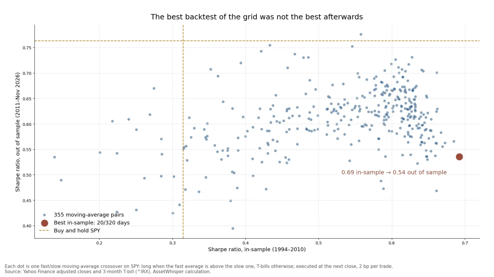
- Overfitting. The best of 355 moving-average pairs on 1994–2010 data ranked 322nd on the years that followed, and the family went from 337 pairs beating buy-and-hold to one.
None of these numbers is a forecast. They are the size of the errors, which is what you need to know to read anyone’s backtest, including your own.
The short answer, in one table
| Error | What the backtest does | Honest result | Flattering result | What to look for |
|---|---|---|---|---|
| Look-ahead | Lets the position earn the move that generated the signal | 9.38% a year (200-day average) | 20.89% a year | When is each trade filled, relative to the data the signal used? |
| Survivorship | Tests today’s index members as if chosen in 2004 | 10.10% a year (RSP) | 16.36% a year | Is the stock universe point-in-time, including companies that later failed or left? |
| Costs | Charges nothing for 45 trades a year | −1.49% a year at 10 bp | 3.00% a year | Turnover per year, times a cost you could defend |
| Overfitting | Reports the best of 355 settings | Sharpe 0.54 out of sample | Sharpe 0.69 in-sample | How many variants were tried, and how the choice did on data it never saw |
All the rules below hold SPY or 3-month Treasury bills, decided at each close, with dividends reinvested and cash earning the T-bill rate. Buy-and-hold SPY over 1994–2026 returned 10.79% a year, with a Sharpe ratio of 0.51 and a worst fall of 55.2%. That is the bar every rule has to clear.
1. Look-ahead bias: trading on information you did not yet have
A moving-average rule computes its signal from the day’s closing price. The commonest coding error is to apply that signal to the same day’s return — to use the day’s move to decide whether you owned the day’s move. It happens whenever the position is not shifted forward, and the fix is one line of code. A milder shortcut is to buy at the very close that produced the signal, which assumes a price known only once the market has shut; the standard used in all our tests is to trade at the next close. The three versions of the same rules:
| Rule, SPY 1994–2026 | Switches a year | Owns the move that made the signal (bug) | Fills at the signal’s close | Fills at the next close |
|---|---|---|---|---|
| Above the 200-day average | 6.5 | 20.89% a year, Sharpe 1.43, worst fall −11.2% | 9.13%, Sharpe 0.58 | 9.38%, Sharpe 0.60, worst fall −22.0% |
| Above the 10-day average | 44.5 | 81.20% a year, Sharpe 5.03, worst fall −5.9% | 3.89%, Sharpe 0.17 | 3.00%, Sharpe 0.10, worst fall −54.6% |
| Hold the day after an up day | 128.1 | 187.35% a year, Sharpe 9.02, no losing day | 3.44%, Sharpe 0.14 | 4.22%, Sharpe 0.20, worst fall −55.9% |
| Buy and hold | — | 10.79% a year, Sharpe 0.51, worst fall −55.2% | ||
The bug, not the shortcut, is what produces impossible results: filling at the signal’s own close moved the 200-day rule by a quarter of a point, while owning the signal’s move added 11.5 points a year. The faster the rule, the bigger the error, because a fast rule’s signal is mostly made of the day’s own move. The last row is the extreme case: with look-ahead, “hold on up days” holds stocks only on days they rose, so it never loses. Real results are rarely that obvious, which is the danger. A 200-day rule showing 21% a year and an 11% worst fall looks like a brilliant discovery rather than a bug.
Look-ahead comes in quieter forms too: fundamental data stamped with the period it describes rather than the date it was published, index membership taken from today’s list, volatility or z-scores computed over the whole sample, and prices adjusted for splits and dividends using information from later dates (harmless for returns, harmful for rules that use price levels). What to look for: the backtest should say when every input became known and when every trade was filled. If it does not, assume the worst. A Sharpe ratio above 1.5 on a single index is itself a reason to check.
2. Survivorship bias: testing the winners after the race
Any stock-picking backtest needs a universe — the stocks it is allowed to choose from. The easy one to download is today’s index. The problem is that today’s S&P 500 is, by construction, the companies that grew enough to be in it now. Firms that shrank, were bought out, went bankrupt or were dropped are missing, and they are missing precisely because they did badly.
To measure it, we took the 503 current members, downloaded their prices back to 2004, and held them in equal weights, rebalanced monthly, from February 2004. The comparison is RSP, the Invesco S&P 500 Equal Weight ETF, which held the actual equal-weighted index over the same period, with the members it had at the time.
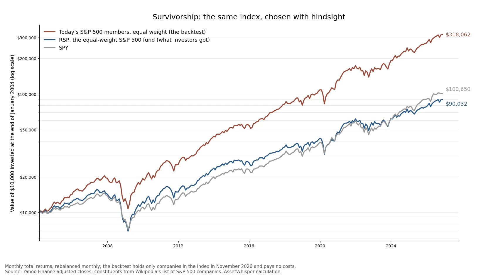
| February 2004 – November 2026 | A year | $10,000 became |
|---|---|---|
| Today’s members, equal weight (the backtest) | 16.36% | $318,062 |
| RSP, the equal-weight S&P 500 fund | 10.10% | $90,032 |
| SPY | 10.64% | $100,650 |
The gap is 6.3 percentage points a year, and it is not a few lucky years: the backtest beat the real fund in every one of the 23 calendar years, by between 0.8 points (2022) and 10.8 points (2007). RSP’s 0.20% expense ratio explains a sliver of it. The rest is hindsight. A stock-selection rule tested on this universe starts with a 6-point head start before it selects anything, which is larger than the edge most published strategies claim.
Only 373 of today’s 502 members with price data were trading in January 2004; the others enter the backtest from their first price, often years before they joined the index, which adds a second layer of hindsight. What to look for: a point-in-time universe — the index as it was on each date, including the companies later removed — and delisted stocks with their final returns. Survivorship does not arise in a test of a single ETF such as SPY, which is why the other three experiments here use one.
3. Costs: the trade you did not pay for
Every switch between stocks and cash costs a spread and some slippage, even at a zero-commission broker. A backtest that charges nothing assumes these are zero. Trading at the next close, here is what each rule earned at different costs per trade:
| Rule, SPY 1994–2026 | Switches a year | 0 bp | 2 bp | 5 bp | 10 bp | 20 bp |
|---|---|---|---|---|---|---|
| 200-day average | 6.5 | 9.38% | 9.24% | 9.02% | 8.67% | 7.96% |
| 10-day average | 44.5 | 3.00% | 2.08% | 0.73% | −1.49% | −5.78% |
| Hold after an up day | 128.1 | 4.22% | 1.58% | −2.25% | −8.32% | −19.35% |
The arithmetic is simple enough to do in your head: annual cost is roughly switches a year times cost per switch. At 44.5 switches and 10 basis points that is about 4.5 points a year, more than the 10-day rule’s 3.0% before costs. A slow rule barely notices costs; a fast one lives or dies on them. None of the three beat buy-and-hold even at zero cost, which is the first thing the costs table should be read against. What to look for: the turnover figure, and costs taken from the spreads on the instruments actually traded, not from a broker’s commission schedule.
4. Overfitting: the best of many tries
The most common way to produce an impressive backtest is not to cheat but to try. We tested every fast/slow moving-average crossover with a fast average of 5 to 100 days and a slow average of 20 to 400 days, in steps of 5 and 20 — 355 pairs — on SPY from 1994 to 2010, trading at the next close and paying 2 basis points a trade. Then we took the pair with the best in-sample Sharpe ratio and ran it, unchanged, on January 2011 to November 2026.
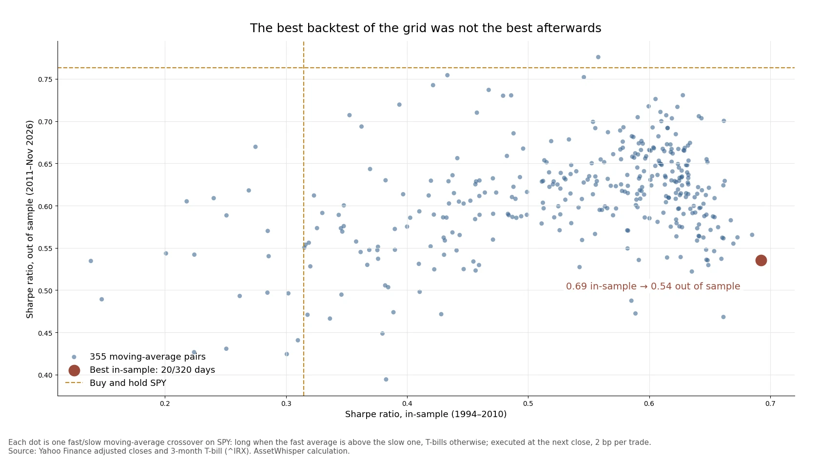
| 1994–2010 (in-sample) | 2011–Nov 2026 (out of sample) | |
|---|---|---|
| Best in-sample pair (20/320 days), Sharpe | 0.69 | 0.54 |
| Best pair, a year | 12.44% | 8.64% |
| Buy and hold, Sharpe | 0.31 | 0.76 |
| Buy and hold, a year | 7.92% | 13.97% |
| Median of all 355 pairs, Sharpe | 0.58 | 0.61 |
| Pairs beating buy and hold on Sharpe | 337 of 355 | 1 of 355 |
Two different things went wrong, and the second is the one most overfitting discussions miss.
The selection added nothing. Out of sample, the best in-sample pair ranked 322nd of 355. The ten best in-sample pairs averaged a Sharpe ratio of 0.67, and 0.58 afterwards — below the median pair’s 0.61. The rank correlation between in-sample and out-of-sample Sharpe across the grid was +0.24: a little information, not much. Picking the winner of the search bought a worse-than-average setting.
The whole family was fitted to the period. 1994–2010 contained two bear markets of roughly 50% (2000–02 and 2007–09), exactly the conditions in which any trend rule looks good, and buy-and-hold had a Sharpe ratio of only 0.31. In that sample, 337 of the 355 pairs beat it. In 2011–2026, a long bull market with short, sharp falls, buy-and-hold’s Sharpe ratio was 0.76 and one pair beat it. No choice of parameters would have rescued a conclusion like “trend following beats buy-and-hold on risk-adjusted returns”: the evidence for it came from which years were in the sample. The same pattern appears on 72 years of data in our test of 90 indicator variants, and the 92-year record of the 10-month moving average shows where that protection did and did not pay.
What the deflated Sharpe ratio says, and what it cannot
Bailey and López de Prado’s deflated Sharpe ratio asks how high the best of N tries would reach by luck alone, given how much the tries’ Sharpe ratios differ from each other, and whether the winner clears that bar. For this grid, the luck bar rises quickly with the number of tries:
| Variants tried | Annualised Sharpe the best would reach by chance |
|---|---|
| 10 | 0.18 |
| 50 | 0.26 |
| 100 | 0.29 |
| 355 | 0.33 |
The winner’s 0.69 clears 0.33 comfortably: its deflated Sharpe ratio is 0.93, a 93% probability that its true Sharpe ratio was above zero once the search is allowed for. That is correct, and it would not have saved anyone. The test compares the winner with zero, and a rule that holds stocks most of the time will have a positive Sharpe ratio in almost any period. The question that mattered was whether it would beat buy-and-hold in a different market, and no statistic computed on one period answers that. Treat the deflated Sharpe ratio as a necessary test, not a sufficient one, and remember that 355 highly correlated variants are fewer independent tries than the count suggests.
A checklist for reading any backtest
- Timing. Is each trade filled after the data that triggered it was available — at the next open or close, never on the bar that produced the signal?
- Universe. For stock selection, is the universe point-in-time, with delisted companies and their final returns?
- Benchmark. Is the result compared with buy-and-hold of the same asset over the same dates, and with a fixed mix holding the same average amount of stock?
- Costs. What is the turnover, and what cost per trade was charged? Re-run the arithmetic: switches × cost.
- Tries. How many rules, parameters, assets and start dates were tested before this one was shown? If the answer is not given, it was not one.
- Out of sample. Was anything held back and run once, unchanged? Did that period contain different market conditions from the one the rule was chosen on?
- Total return and cash. Are dividends included, and does cash earn a T-bill rate rather than zero?
- Plausibility. A Sharpe ratio above about 1.5 on one index, a worst fall under 10%, or a rule with no losing year are reasons to look for one of the four errors above before believing it.
Any of the libraries in our comparison of Python backtesting libraries can run these checks, and none of them runs them for you. The step-by-step version, with random-timing and naive-mix benchmarks, is in how to test a technical indicator before trusting it; what the main strategy families have earned once these checks are applied is in which algorithmic trading strategies are actually profitable.
Frequently asked questions
What is look-ahead bias in backtesting?
Using information in a simulated trade that would not have been available when the trade was made. The commonest form is a position that is not shifted forward, so that each day’s signal is applied to the return that produced it. On SPY from 1994 to 2026, letting the position earn the move that produced the signal raised a 200-day moving-average rule from 9.4% a year to 20.9%, and a 10-day rule from 3.0% to 81.2%.
What is survivorship bias in backtesting?
Testing on a universe that contains only the companies that survived to today. Today’s S&P 500 members, equal-weighted from 2004, returned 16.4% a year, against 10.1% for the fund that held the equal-weight index as it actually was — a gap of 6.3 points a year, positive in every calendar year.
What is overfitting in a trading strategy?
Choosing rules or parameters because they fitted past data best, so that the result describes the sample rather than the market. The best of 355 moving-average pairs on 1994–2010 data ranked 322nd on 2011–2026. Overfitting can also be to the period: almost every pair beat buy-and-hold in a sample with two bear markets, and almost none in the bull market that followed.
What is a good Sharpe ratio for a backtest?
There is no threshold that makes a backtest trustworthy, because the errors above inflate the Sharpe ratio more than skill does. As a reference, buy-and-hold SPY earned 0.51 from 1994 to 2026. A single-index timing rule showing much more than that, especially above 1.5, should be checked for look-ahead and for the number of variants tried before it is believed.
How many years of data does a backtest need?
More than most people use. The standard error of an annualised Sharpe ratio is roughly √((1 + SR²/2) / years). For a true Sharpe ratio of 0.5 that is about 0.33 with 10 years of data and 0.19 with 30, so ten years cannot reliably tell a 0.5 strategy from a 0.2 one. The period also needs to contain more than one kind of market, as the overfitting test shows.
What is the deflated Sharpe ratio?
A test proposed by David Bailey and Marcos López de Prado in 2014 that adjusts a backtest’s Sharpe ratio for the number of variants tried, the spread of their results, the length of the sample and the shape of the returns. It answers whether the best result is likely to be above zero after the search. It does not answer whether the strategy will beat a benchmark in a different period.
What is walk-forward testing?
Choosing parameters on one window, testing them on the next, then rolling both forward and repeating. It uses more of the data for testing than a single split, but every window still comes from the same history. It reduces parameter overfitting; it cannot remove the dependence on which market conditions the history happened to contain.
How we calculated this
- Data: SPY and RSP dividend-adjusted daily closes and the 13-week Treasury bill yield (^IRX) from Yahoo Finance, to 3 November 2026. Cash earns the T-bill yield divided by 252 each day.
- Rules: long SPY when the close is above its 200-day or 10-day simple moving average, or after a day with a positive return; T-bills otherwise. The standard version applies the position decided at close t to the return from close t+1 to close t+2 (bought at the next close); the shortcut, to the return from t to t+1 (bought at the signal’s close); the bug, to the return ending at close t.
- Costs: each full switch between SPY and T-bills is charged the stated cost once.
- Survivorship: current constituents from Wikipedia’s list of S&P 500 companies (503 tickers; 502 with data), monthly total returns, equal weight across members with a price at the start of each month, February 2004 to November 2026; no costs. RSP’s returns are net of its expense ratio.
- Overfitting: fast averages of 5–100 days in steps of 5 and slow averages of 20–400 days in steps of 20, fast shorter than slow (355 pairs); 2 bp per switch; Sharpe ratios on daily returns in excess of T-bills, annualised by √252. In-sample January 1994 – December 2010; out of sample January 2011 – 3 November 2026.
- Deflated Sharpe ratio: Bailey and López de Prado (2014), using the variance of the 355 in-sample daily Sharpe ratios and the skewness and kurtosis of the best pair’s daily excess returns.
- The calculation script and its output, kept with the article, reproduce every figure.
Sources
- Bailey, D. H. and López de Prado, M., “The Deflated Sharpe Ratio: Correcting for Selection Bias, Backtest Overfitting and Non-Normality”, Journal of Portfolio Management, 40(5), 2014.
- Bailey, D. H., Borwein, J., López de Prado, M. and Zhu, Q. J., “Pseudo-Mathematics and Financial Charlatanism: The Effects of Backtest Overfitting on Out-of-Sample Performance”, Notices of the American Mathematical Society, 61(5), 2014.
- Lo, A. W., “The Statistics of Sharpe Ratios”, Financial Analysts Journal, 58(4), 2002 — standard error of the Sharpe ratio.
- Prices: Yahoo Finance via yfinance, retrieved 4 November 2026. Constituents: Wikipedia, List of S&P 500 companies, retrieved 4 November 2026.
Related reading
- How to test a technical indicator before trusting it — the six-step test, run on 90 rule variants.
- Python backtesting libraries in 2026 — which engine to run the checks in.
- The 10-month moving average on the S&P 500 — 92 years of the rule used here.
- Which algorithmic trading strategies are actually profitable? — the strategy families, after costs.
- The Sharpe ratio — the statistic every backtest reports, and its limits.
This article is general information, not personalised investment advice. It does not take into account the financial situation, objectives or risk tolerance of any individual reader, and the same text is distributed to all readers. The rules tested are illustrations of backtesting errors, not trading recommendations. Past performance, real or simulated, does not indicate future results, and capital is at risk.