vectorbt in Practice: a Reproducible Backtest from Raw Data to Report
Key takeaway
With its default settings, vectorbt reports that buying and holding SPY since 1993 returned 15.8% a year; the real figure is 10.6%. A complete, reproducible vectorbt backtest of a 200-day moving-average rule, with frozen data, every setting that changes the answer measured, and an out-of-sample test in which none of 29 windows beat buy-and-hold after 2010.
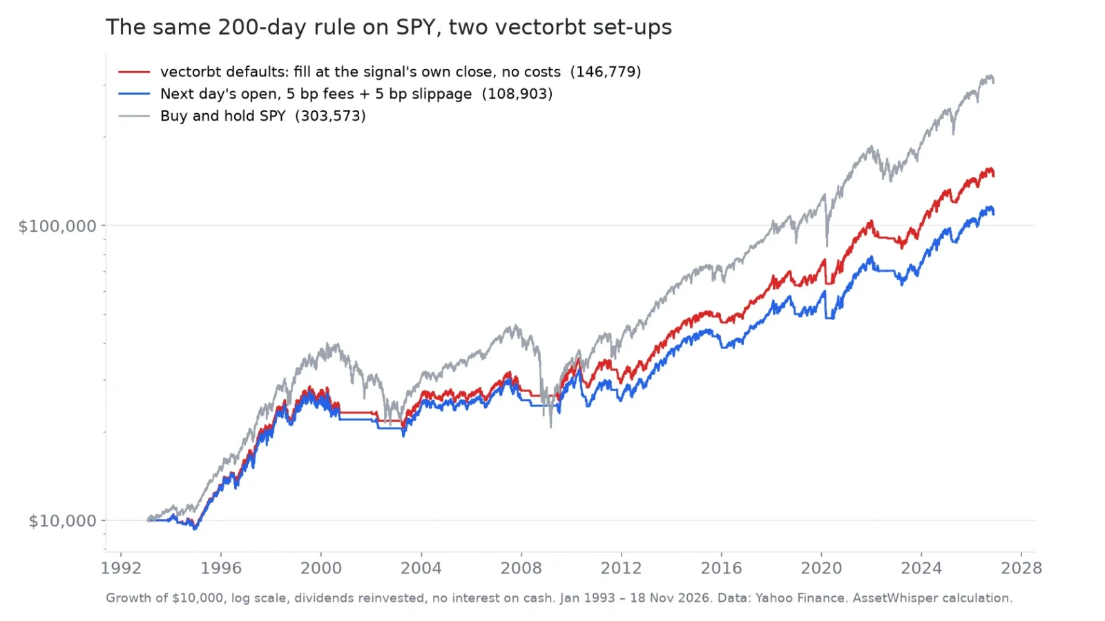
Run with its default settings, vectorbt reports that buying and holding SPY since 1993 returned 15.8% a year. The real figure is 10.6%. Nothing is wrong with the library’s arithmetic: it is doing exactly what its defaults tell it to do, and one of those defaults does not fit daily stock-market data.
This is a complete, reproducible vectorbt backtest, from downloading prices to reading the report, with every setting that changes the answer measured on the same rule. The rule is deliberately boring: hold SPY while its close is above its 200-day moving average, otherwise hold cash. The point is the workflow, not the rule.
- The year length inflates every annualised number. vectorbt assumes a 365-day year, while the data has about 252 trading days a year. Left as it is, SPY’s annualised return comes out at 15.76% instead of 10.62%, its volatility at 22.3% instead of 18.5%, and its Sharpe ratio at 0.77 instead of 0.64.
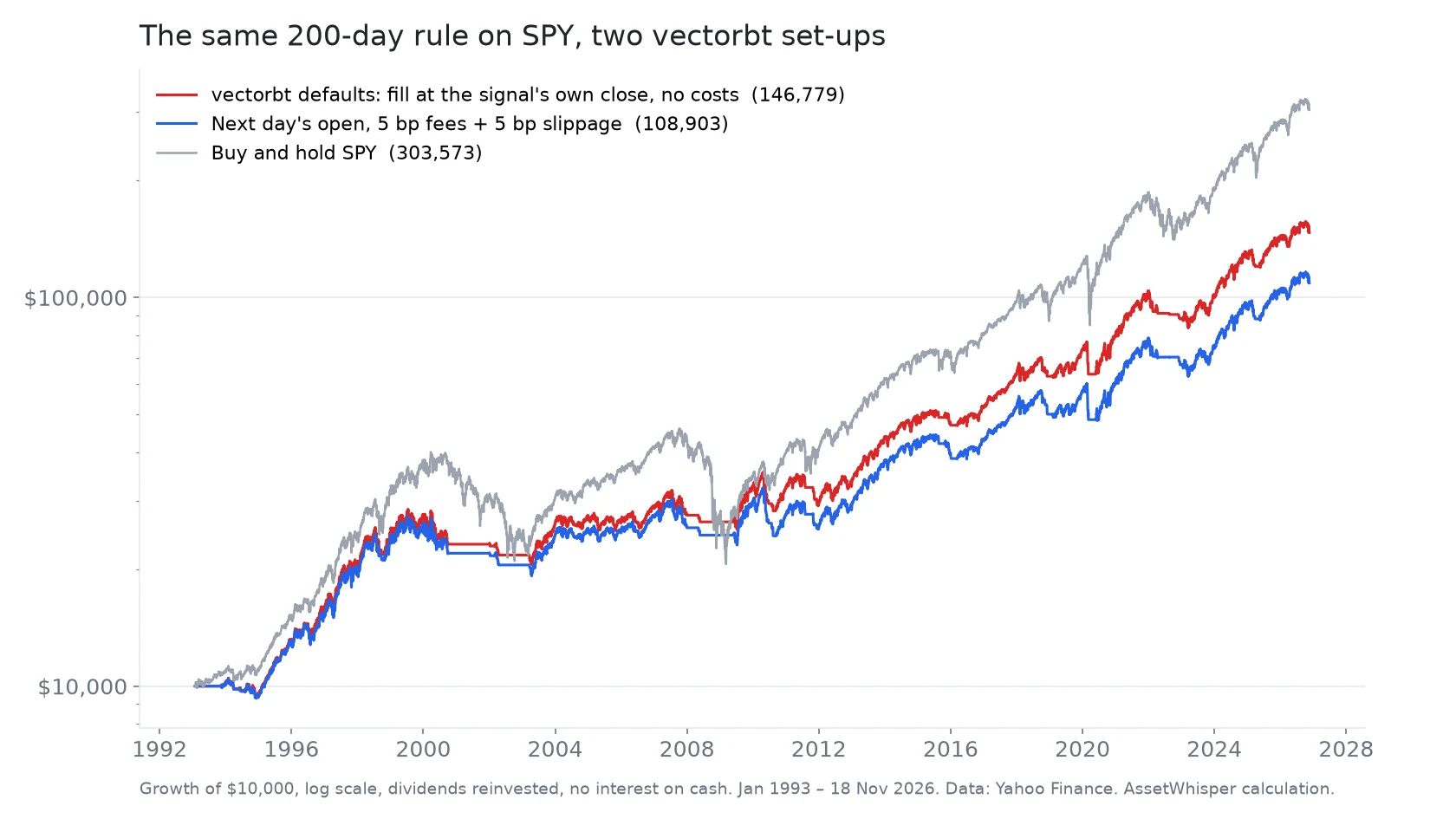
- Fill timing and costs take a third off the end result. With the defaults, $10,000 in the rule became $146,779. Acting at the next day’s open and paying 5 basis points of fees and 5 of slippage on every order, it became $108,903: 7.32% a year instead of 8.27%.
- vectorbt pays nothing on cash. The rule was out of the market on 24.4% of days. Crediting the Treasury bill rate on those days lifts it to 7.90% a year.
- The parameter search is fast, and it is where the danger is. 29 moving-average lengths ran in 0.02 seconds. The best one on 1994–2009 data held up well on 2010–2026, but none of the 29 beat buying and holding SPY over 2010–2026, on return or on Sharpe ratio.
The data, the code and its output are fixed, so anyone running the same script gets the same numbers. None of this is a recommendation of the rule, which is used only as a test case.
The short answer, in one table
| SPY, 29 Jan 1993 – 18 Nov 2026, 200-day moving-average rule | Growth of $10,000 | Return a year | Maximum drawdown |
|---|---|---|---|
| vectorbt defaults: filled at the close that triggered the signal, no costs | $146,779 | 8.27% | −28.0% |
| Filled at the signal’s close, 5 bp fees + 5 bp slippage | $118,384 | 7.59% | −30.8% |
| Filled at the next day’s open, no costs | $135,024 | 8.00% | −27.1% |
| Filled at the next day’s open, 5 bp fees + 5 bp slippage | $108,903 | 7.32% | −30.0% |
| Same, with the Treasury bill rate earned on cash | $130,540 | 7.90% | −24.9% |
| Buy and hold SPY | $303,573 | 10.62% | −55.2% |
Returns a year are compounded over calendar time, 33.8 years. Dividends reinvested, no taxes. 108 trades in every version of the rule.
What you need
vectorbt is a Python library that runs a backtest on whole arrays at once instead of looping bar by bar, which is what makes it fast. Version 1.2.0, released on 19 October 2026, supports Python 3.11 to 3.14. Its licence is Apache 2.0 with the Commons Clause added, which rules out selling a product whose value comes substantially from vectorbt itself; we compared it with Backtrader and backtesting.py, and their licences, in Python backtesting libraries in 2026.
Pin every version. vectorbt depends on pandas, NumPy and Numba, and a change in any of them can move a result. This article was run with:
# requirements.txt
vectorbt==1.2.0
pandas==3.1.1
numpy==2.5.5
numba==0.68.1
yfinance==1.8.0
matplotlib==3.11.2
# Python 3.12.12
Step 1: download the data once, then freeze it
The most common reason a backtest cannot be reproduced is not the code, it is the data. Dividend-adjusted prices are recalculated every time a fund pays a dividend: each payment scales down every price before it, so that the series shows total return. SPY’s dividend of $1.889 on 18 September 2026 multiplied 8,466 of the 8,510 adjusted closes in our sample by 0.997523. The first close in the series, $43.94 as traded on 29 January 1993, is now $24.05 adjusted. Download the same series in December and every historical price will have moved again.
So the download happens once, the result is saved to a file, and the file gets a fingerprint:
import hashlib
import pandas as pd
import yfinance as yf

px = yf.download("SPY", start="1990-01-01", end="2026-11-19", auto_adjust=True, progress=False)
px.columns = px.columns.get_level_values(0)
px[["Open", "High", "Low", "Close", "Volume"]].to_csv("spy_adjusted.csv", float_format="%.6f")

print(hashlib.sha256(open("spy_adjusted.csv", "rb").read()).hexdigest())
# e1bf99e0213a92e8ffddae46deb041040c7dd42cf5a0bfb1ebdf83f36a8e4d89

df = pd.read_csv("spy_adjusted.csv", index_col=0, parse_dates=True)   # from here on, only the file
close, open_ = df["Close"], df["Open"]
Two details matter here. auto_adjust=True adjusts the open, high and low as well as the close, so the open used for fills later is on the same scale as the close used for signals. And the hash goes in the report: if someone gets a different fingerprint, they know before running anything that their numbers will differ.
Free data has a second limit that no setting fixes: SPY is a fund that has existed since 1993, so it has no survivorship problem, but a list of today’s stocks downloaded from the same source does. How much that bias is worth is measured in how to read a backtest: 6.3 percentage points a year on the S&P 500 since 2004.
Step 2: turn the rule into entries and exits
import vectorbt as vbt

vbt.settings.returns["year_freq"] = "252 days"   # why: step 4

ma = vbt.MA.run(close, 200).ma
above = close > ma
entries = above & ~above.shift(1, fill_value=False)   # first day above the average
exits = ~above & above.shift(1, fill_value=False)     # first day back below
The average needs 200 closes before it exists, so the first possible signal is on 11 November 1993. Until then above is false, and the rule holds cash. Over the whole sample the rule crossed the line 215 times: 108 entries and 107 exits, with the last position still open on 18 November 2026.
Step 3: the portfolio, and the three defaults to change
The shortest possible call works, and it is what most tutorials show:
pf_default = vbt.Portfolio.from_signals(close, entries, exits, freq="1D")Behind it are three defaults that make a backtest look better than anything that could be traded:
- The fill price is the close of the signal bar. The signal needs that close to exist, so the trade happens at a price that was only known once it could no longer be traded at. On the 215 signal days, SPY’s next open was on average 0.51% away from the close that triggered the signal. This is the look-ahead problem in its mildest form.
- Fees and slippage are zero.
- Starting cash is $100 and each entry uses all of it (
sizeis infinite). That is harmless here, but the report’s dollar figures, such as fees paid and expectancy, are then in hundreds of dollars and easy to misread.
The version we would trust shifts the signals by one bar, fills at that bar’s open, and charges every order:
pf = vbt.Portfolio.from_signals(
    close,
    entries.shift(1, fill_value=False),   # act on the next bar...
    exits.shift(1, fill_value=False),
    price=open_,                          # ...at its open
    fees=0.0005,                          # 5 bp of the order value
    slippage=0.0005,                      # 5 bp worse than the open
    init_cash=10_000,
    freq="1D",
)
Of the 0.95 percentage points a year between the default and this version, 0.27 came from the fill timing and 0.68 from costs. The fees alone came to $3,579 on a $10,000 start, before slippage. SPY is among the cheapest securities in the world to trade; on a small-cap stock or a crypto pair the same rule would pay several times more. How fast costs grow with trading frequency is in how to read a backtest, where 10 basis points a trade sank a rule that traded 45 times a year.
Step 4: the report, and the setting that inflates it
pf.stats() prints the full report in one line. Before trusting it, check one setting: year_freq, the length of a year that vectorbt uses to annualise. Its default is 365 days. With freq="1D", that tells vectorbt each bar is one day and a year has 365 of them, but stock-market data has a bar only on trading days, about 252 a year (251.8 in this sample). vectorbt then thinks 8,510 bars are 23.3 years, when they are 33.8.
| What vectorbt reports | Buy and hold, default year (365 days) | Buy and hold, year_freq="252 days" |
The rule, default year | The rule, 252 days |
|---|---|---|---|---|
| Annualised return | 15.76% | 10.64% | 10.78% | 7.33% |
| Annualised volatility | 22.30% | 18.53% | 14.50% | 12.05% |
| Sharpe ratio | 0.768 | 0.638 | 0.779 | 0.647 |
| Sortino ratio | 1.093 | 0.908 | 1.078 | 0.896 |
| Calmar ratio | 0.286 | 0.193 | 0.360 | 0.244 |
The true compound returns, from calendar dates, are 10.62% and 7.32%. With the default, the rule’s annualised return comes out above the true return of buying and holding, which is the kind of mistake that ends up in a presentation.
Ratios scaled by the square root of the year, like Sharpe and Sortino, are overstated by about 20% (the square root of 365/252); returns and Calmar by more. The fix is the one line in step 2, set before anything is computed. vectorbt also caches the results of its metrics, so changing the setting after calling pf.sharpe_ratio() may not change the next call: set it at the top of the script. If freq is left out altogether, vectorbt cannot work out the bar length from a trading-day index and refuses to compute any annualised figure, which is better than a wrong one.
With the setting fixed, the report for the rule against buying and holding:
From pf.stats() |
200-day rule, next open, with costs | Buy and hold SPY |
|---|---|---|
| Total return | 989% | 2,936% |
| Maximum drawdown | 30.0% | 55.2% |
| Longest drawdown, as reported | 1,865 days | 1,656 days |
| Longest drawdown, in fact | July 1999 – December 2006 (7.4 years) | March 2000 – October 2006 (6.6 years) |
| Trades | 108 | 1 |
| Win rate (closed trades) | 27.1% | — |
| Average winning / losing trade | +14.36% / −1.60% | — |
| Profit factor | 3.16 | — |
| Fees paid (excluding slippage) | $3,579 on $10,000 | $0 |
| Sharpe ratio | 0.647 | 0.638 |
| Sortino ratio | 0.896 | 0.908 |
| Calmar ratio | 0.244 | 0.193 |
Read together, the numbers describe a typical trend rule: it lost on almost three trades in four, small and quickly, and made its money on a few long holdings. It cut the worst fall from 55% to 30% and ended with a third of the money. Its Sharpe ratio is level with buying and holding. vectorbt’s Sharpe ratio uses a risk-free rate of zero unless told otherwise, and so does every ratio in this article; the difference between Sharpe, Sortino and Calmar, and when each misleads, is in our article on the Sharpe ratio.
The same freq setting hides a second trap in the durations. vectorbt counts bars and labels them days, so its “1,865 days” of drawdown are 1,865 trading days: from July 1999 to December 2006, 7.4 years on the calendar, not 5.1. Average trade durations in the report are trading days too.
The longest drawdown is longer for the rule than for buying and holding, even though it is about half as deep. A rule that steps aside in a fall also misses the first part of the recovery: after the 2000–2002 bear market, buying and holding was back at its high in October 2006 and the rule only in December 2006.
Step 5: what vectorbt leaves out
The library models the trades. It does not model what the money does between them. While the rule is out of the market, its cash earns nothing, which understates any rule that spends time in cash. The fix is a few lines outside vectorbt, with a Treasury bill series saved and fingerprinted like the prices:
irx = pd.read_csv("irx.csv", index_col=0, parse_dates=True)["Close"]   # ^IRX, 13-week T-bill, frozen
rf = (irx.reindex(close.index).ffill() / 100 / 252).fillna(0)
r_cash = pf.returns() + rf.where(~pf.position_mask(), 0)
print(10_000 * (1 + r_cash).prod())   # 130,540
Out of the market on 24.4% of days, the rule earned 0.58 percentage points a year more with interest on its cash: 7.90% instead of 7.32%, still 2.7 points a year below buying and holding. The approximation credits the bill rate for each full day in cash and ignores interest on the partial days around a trade, which is small at 108 trades.
Two other things are outside the model and need to be stated in any report. Taxes: every exit realises a gain in a taxable account, and buying and holding defers them. And dividends: the adjusted series reinvests them on the ex-date at no cost, which slightly flatters both lines.
Step 6: test many parameters in one call
This is what vectorbt is built for. Passing a list of windows instead of one number returns one column per window, and the portfolio runs every column at once:
windows = list(range(20, 301, 10))                 # 29 lengths
ma_grid = vbt.MA.run(close, windows).ma            # one column per window
above_g = ma_grid.rsub(close, axis=0) > 0          # close above each average
prev = above_g.shift(1, fill_value=False)

pf_grid = vbt.Portfolio.from_signals(
    close,
    (above_g & ~prev).shift(1, fill_value=False),
    (~above_g & prev).shift(1, fill_value=False),
    price=open_, fees=0.0005, slippage=0.0005, init_cash=10_000, freq="1D",
)
The 29 backtests of 8,510 days each ran in 0.02 seconds on a laptop, after Numba’s first compilation. The 200-day column matches the single run of step 3 to the cent, which is a check worth keeping in any script: a grid that does not reproduce its own single case has a bug.
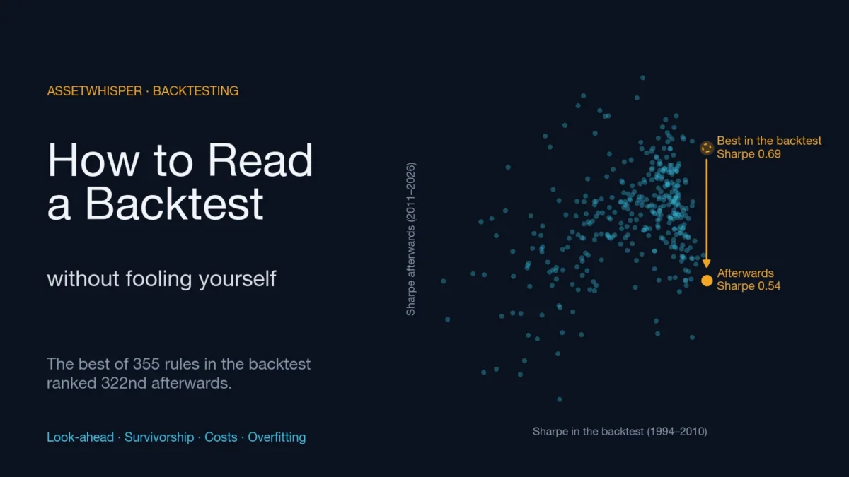
The speed is the risk. Testing a thousand variants is as easy as testing one, and the best of a thousand will look good by chance alone. In how to read a backtest, the best of 355 moving-average pairs on old data ranked 322nd on new data. The only defence is to keep part of the data out of the search.
Step 7: choose on old data, test on new data
We split the sample at 1 January 2010. Each window was scored on April 1994 to December 2009, the first date on which all 29 averages exist, and the one with the best Sharpe ratio was then run, unchanged, on 2010 to November 2026:
r = pf_grid.returns().iloc[301:]          # every window has its average from here

def sharpe(x):
    return x.mean() / x.std() * 252 ** 0.5

s_in, s_out = sharpe(r.loc[:"2009"]), sharpe(r.loc["2010":])
best = s_in.idxmax()
print(best, s_in[best], s_out[best], s_out.rank(ascending=False)[best])
# 290  0.819  0.766  2.0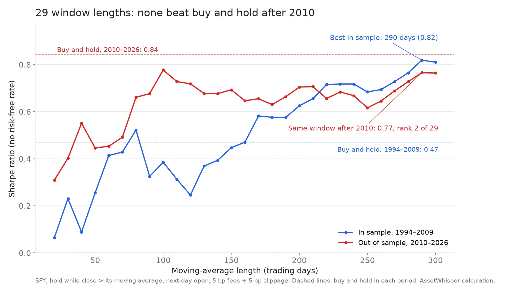
The result is less dramatic than the 355-pair example, and more useful for it:
- The winner held up. The 290-day average had the best Sharpe ratio before 2010 (0.82) and the second best after (0.77). The ranking carried over in part: the rank correlation between the two periods was 0.40. Long windows did better than short ones in both periods, which is a broad pattern, not a single lucky number.
- The whole family lost to the benchmark. After 2010, buying and holding SPY had a Sharpe ratio of 0.84 and returned 13.76% a year. Not one of the 29 windows matched it on either measure; the best returned 9.6% a year. Before 2010 the long windows beat buying and holding on Sharpe ratio (0.47), because that period held two falls of about 50%. The rule did what it does, cutting drawdowns, and the period after 2010 rewarded staying in.
- Re-optimising every year added nothing. Choosing the window each January by its Sharpe ratio over the previous ten years, from 2005 to 2026, gave a Sharpe ratio of 0.61 and 6.81% a year. Keeping the 200-day average fixed over the same years gave 0.63 and 6.88%. The yearly choice switched between six windows.
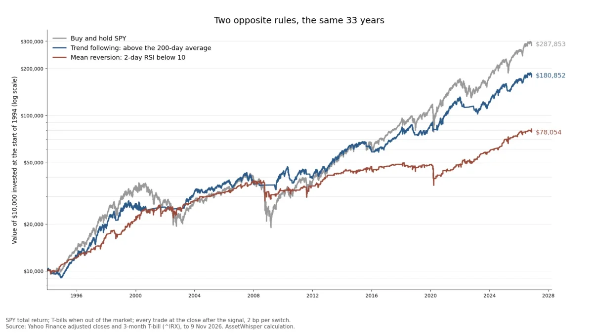
A split test does not prove a rule works; it only catches some of the ways a rule can fail. The six checks we apply before trusting any indicator are in how to test a technical indicator, and this same 200-day rule is set against a short-term mean-reversion rule in mean reversion vs trend following.
A checklist for a reproducible vectorbt backtest
- Versions pinned in a requirements file, Python version included.
- Data saved to a file with its SHA-256 hash, and the script reading only the file after the first download.
freqandyear_freqset at the top:"1D"and"252 days"for daily stock data; for crypto, which trades every day, 365 is right. Durations in the report are then in trading days, whatever the label says.- Signals shifted one bar and filled at the next open, unless the strategy really trades at the close with an order placed before it.
- Fees and slippage on every order, at a level that fits the instrument, and a second run with double the costs.
- Cash interest, taxes and dividend treatment stated, added outside the library where they matter.
- The grid checked against one single run, and the parameter chosen on data that the final test does not use.
- A benchmark in the same report, run with the same settings.
- The output saved next to the script, so a reader can check a figure without running anything.
Frequently asked questions
Why is vectorbt’s annualised return so high?
Usually because of the year length. vectorbt annualises with a 365-day year by default, while daily stock data has about 252 bars a year. On SPY from 1993 to November 2026 that turned a 10.62% compound return into a reported 15.76%. Setting vbt.settings.returns["year_freq"] = "252 days" at the top of the script gives 10.64%.
Does vectorbt avoid look-ahead bias?
Not by default. Portfolio.from_signals fills at the close of the bar on which the signal appears, a price that was known only at the moment it could no longer be traded at. Shift the entries and exits by one bar and pass the next bar’s open as price. On the 200-day rule on SPY, that changed the result by 0.27 percentage points a year.
How do I add fees and slippage in vectorbt?
With the fees and slippage arguments of Portfolio.from_signals, both as fractions: 0.0005 is 5 basis points. Fees are charged on the value of each order, and slippage moves the fill price against the trade. 5 basis points of each cost the 200-day rule 0.68 percentage points a year over 215 orders.
Does vectorbt include interest on cash?
No. Cash earns nothing while the strategy is out of the market. Add the Treasury bill return on the days with no position, using pf.position_mask(). For the 200-day rule, out of the market on 24.4% of days since 1993, that added 0.58 percentage points a year.
Is vectorbt free to use?
The open-source version is, under Apache 2.0 with the Commons Clause, which rules out selling a product or service whose value comes substantially from vectorbt. A separate paid version, vectorbt PRO, is not covered here.
How do I avoid overfitting a parameter grid in vectorbt?
Choose the parameter on one part of the data and test it, unchanged, on a later part the search never saw. On SPY, the best of 29 moving-average lengths on 1994–2009 ranked second of 29 on 2010–2026, but none of the 29 beat buying and holding over 2010–2026.
How we calculated this
- Data: SPY daily open, high, low and close from Yahoo Finance via yfinance, dividend-adjusted (
auto_adjust=True), 29 January 1993 to 18 November 2026, 8,510 bars; unadjusted closes and dividends for the adjustment example; 13-week Treasury bill yield (^IRX) for the cash leg. Downloaded on 19 November 2026 and saved with their SHA-256 hashes. - Rule: long when the close is above its 200-day simple moving average, otherwise flat. Entry and exit on the first day of each crossing. The realistic set-up acts on the open of the next trading day, with fees of 5 basis points and slippage of 5 basis points on every order, all available cash invested.
- Returns a year in the tables are compounded over calendar time (33.8 years for the full sample). Sharpe ratios use daily returns, no risk-free rate, and √252.
- Cash interest: the daily bill rate (yield / 252) added on every day without a position.
- Grid: 29 windows from 20 to 300 days in steps of 10, same execution. In sample: 8 April 1994 (the first day with all averages live) to 31 December 2009. Out of sample: 4 January 2010 to 18 November 2026. Walk-forward: each January from 2005, the window with the best Sharpe ratio over the previous ten years, held for that year.
- Timing is the median of five runs in one process on an Apple M1 Pro laptop, after a first run to compile Numba’s functions.
- Run with Python 3.12.12, vectorbt 1.2.0, pandas 3.1.1, NumPy 2.5.5 and Numba 0.68.1. The script and its full output, kept with the article, reproduce every figure.
Sources
- vectorbt, source code and licence (version 1.2.0) and documentation:
Portfolio.from_signalsand thereturnssettings. - Yahoo Finance, SPY and ^IRX daily history, through the yfinance package (version 1.8.0), downloaded on 19 November 2026.
- David H. Bailey, Jonathan M. Borwein, Marcos López de Prado and Qiji Jim Zhu, “Pseudo-Mathematics and Financial Charlatanism: The Effects of Backtest Overfitting on Out-of-Sample Performance”, Notices of the American Mathematical Society, May 2014.
Related reading
- How to read a backtest without fooling yourself — look-ahead, survivorship, costs and overfitting, each measured.
- Python backtesting libraries in 2026 — vectorbt against Backtrader and backtesting.py on the same prices.
- The 10-month moving average on the S&P 500 — 92 years of the rule used here, in its monthly form.
- Mean reversion vs trend following — the 200-day average against a 2-day RSI rule on SPY.
- How to test a technical indicator — the six checks before trusting a rule.
This article is general information, not personalised investment advice. It does not take into account the financial situation, objectives or risk tolerance of any individual reader, and the same text is distributed to all readers. The moving-average rule is a test case for the software, not a recommendation. Past performance, real or simulated, does not indicate future results, and capital is at risk.