How to Test a Technical Indicator Before Trusting It: 90 Rule Variants Against a Naive Benchmark
Key takeaway
On the S&P 500 from 1954 to 2026, with costs and next-day execution, none of four common indicator rules or 90 variants of them beat buy-and-hold on return after 1992. MACD and TRIX lost to a same-exposure stock-and-bill mix in both periods; the 200-day average kept a better Sharpe ratio, not a return edge.

Most indicator backtests answer the wrong question. They ask whether a rule made money, and in a market that rose for most of a century almost any rule that owns stocks part of the time did. The question that decides whether an indicator is worth anything is narrower: did it beat a rule that needs no indicator at all? We used two: holding the S&P 500, and holding a fixed mix of the index and Treasury bills with the same average amount of stock as the indicator rule.
We ran that test on four of the most quoted rules, the 200-day moving average, MACD, RSI and TRIX, and on 90 variants of them, from January 1954 to September 2026, with trading costs and every trade made at the close after the signal. The years from 1993 on were held out: no rule or setting was chosen on them. None of the 90 variants beat buy-and-hold on return after 1992. MACD and TRIX lost to the naive mix in both halves of the sample. The 200-day average beat it by 2.4 points a year before 1993 and by 0.1 points after; what survived was a higher Sharpe ratio and, on this one historical path, a shallower worst fall, not a higher return.
The short answer, in one table
The held-out years, January 1993 to September 2026. Each rule holds the S&P 500 with dividends when its signal is on and 3-month Treasury bills when it is off, paying 5 basis points (0.05%) per switch. The naive mix holds the rule’s average share in stocks every day.
| 1993–Sep 2026 | In stocks | Return a year | Naive mix | Sharpe | Worst fall |
|---|---|---|---|---|---|
| Buy and hold | 100% | 10.89% | n/a | 0.52 | −55.3% |
| 200-day average | 76% | 9.20% | 9.14% | 0.60 | −21.7% |
| MACD 12-26-9 | 50% | 2.94% | 7.12% | 0.09 | −35.3% |
| RSI 14, 30/70 | 35% | 7.40% | 5.79% | 0.38 | −51.5% |
| TRIX 15, 9 | 49% | 5.99% | 6.99% | 0.35 | −27.1% |
A fixed stock-and-bill mix has about the index’s Sharpe ratio (0.51 to 0.52 here), because it only scales risk, so the Sharpe column compares each rule with a naive portfolio of the same risk. The 200-day average matched its mix’s return with a higher Sharpe ratio and half its worst fall (−21.7% against −44.3%). RSI beat its mix’s return with more risk and a lower Sharpe ratio. MACD earned less than half of what its mix did; TRIX a point a year less.
Step 1: fix the rule, and trade it the day after
The four rules use textbook settings, fixed before any data was loaded:
- 200-day average: in stocks when the index closes above the simple average of its last 200 closes.
- MACD 12-26-9: in stocks when the 12-day minus the 26-day exponential average is above its own 9-day exponential average.
- RSI 14, 30/70: in stocks from the day the 14-day relative strength index falls below 30 until it rises above 70.
- TRIX 15, 9: in stocks when the daily rate of change of a triple-smoothed 15-day exponential average is above its own 9-day exponential average.
Every signal is computed at a close and executed at the next close. Trading at the close that produced the signal assumes a price only known once the market has shut, and how much that matters varies from rule to rule. The shortcut turned MACD, which switches about 20 times a year, from a rule that trailed its naive mix by 1.0 point a year over 1954–1992 into one that beat it by 2.0 points. For the 200-day average the difference was under 0.7 points either way. For a monthly rule it is smaller still: the 10-month average in our 92-year study takes its position at the month-end close, as the SPY backtest in our review of algorithmic trading strategies, which has the general checklist, does in most months; in our daily replica of that rule, moving the trade to the next close changed its return by less than 0.4 points a year in either half of our sample.
Step 2: beat buy-and-hold, then beat the naive mix
A rule that is out of the market half the time has lower volatility and a smaller worst fall than buy-and-hold even with random timing, because it owns less stock. The fair comparison is a fixed mix with the same average share in stocks, rebalanced daily: the rule with the timing taken out.
| Edge over naive mix | 1954–1992 | 1993–2026 | Sharpe, before | Sharpe, after |
|---|---|---|---|---|
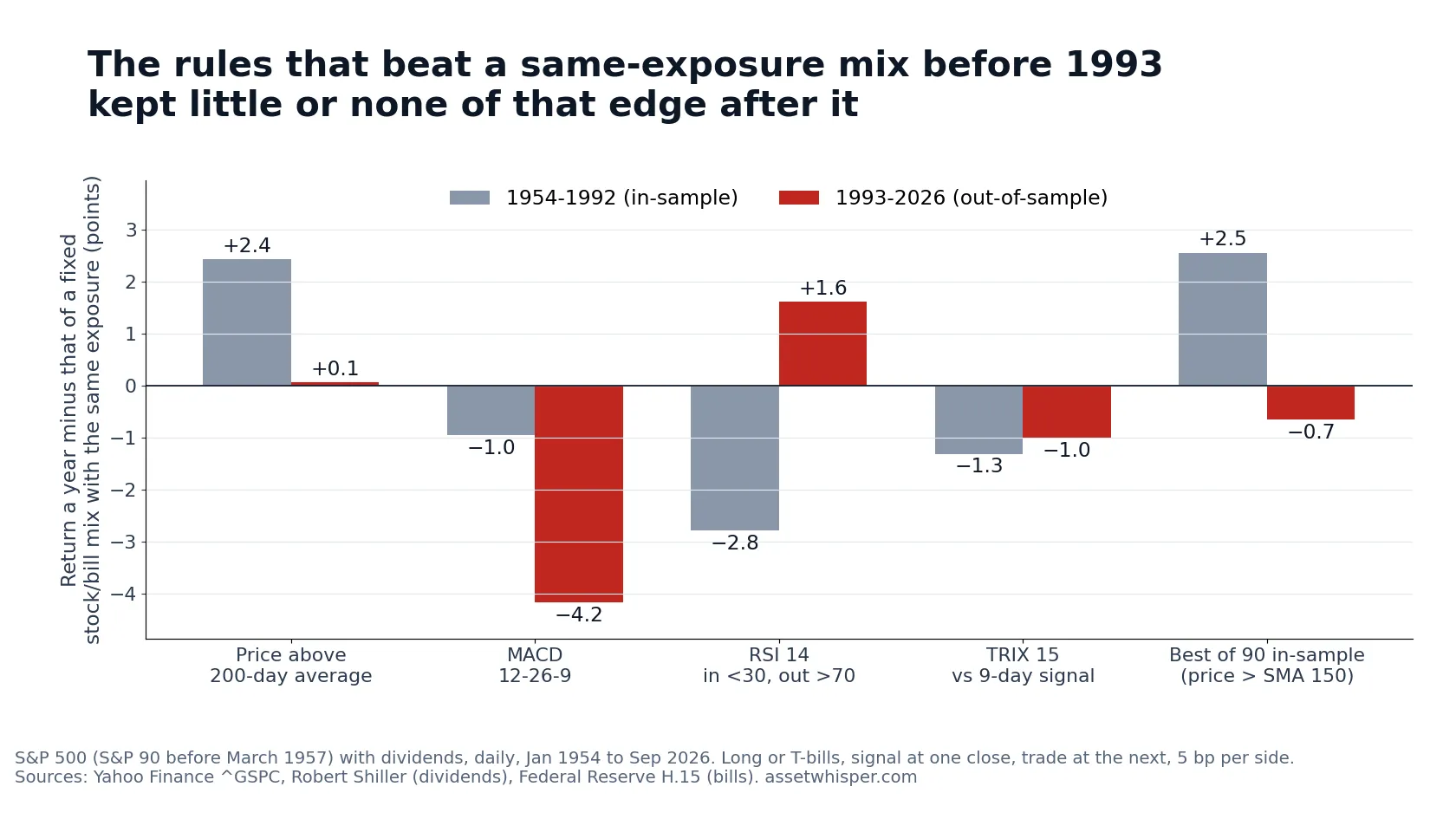
| 200-day average | +2.42 | +0.06 | 0.67 vs 0.45 | 0.60 vs 0.52 |
| MACD 12-26-9 | −0.96 | −4.18 | 0.27 vs 0.45 | 0.09 vs 0.51 |
| RSI 14, 30/70 | −2.80 | +1.61 | 0.02 vs 0.45 | 0.38 vs 0.51 |
| TRIX 15, 9 | −1.31 | −1.00 | 0.23 vs 0.45 | 0.35 vs 0.51 |
Edges are points of return a year after costs. Before 1993 the 200-day average passed both tests: it beat buy-and-hold (12.48% a year against 11.74%, with a worst fall of 16.5% against 45.0%) and its naive mix. MACD and TRIX failed against their mix in both periods, and the mix also had the higher Sharpe ratio in both. RSI reversed. The worst of the four before 1993, it beat its mix on return afterwards while invested in the most violent markets: the index’s volatility was 25% on its in-market days, against 13% on the others.
Step 3: beat random timing with the same trades
A stricter benchmark trades exactly as often, and stays in exactly as long, but at random: we shuffled the order of each rule’s own in-market and out-of-market spells 1,000 times, keeping its days in stocks, trades and costs.
- 200-day average: before 1993 its Sharpe ratio beat 997 of the 1,000 random versions and its return 977. After 1992 its Sharpe ratio still beat 976 and its worst fall was shallower than all 1,000, but its return beat only 744.
- MACD: after 1992, 962 of the random versions earned at least as much.
- TRIX: a coin toss on return (it beat 367 random versions before 1993 and 529 after), although after 1992 its worst fall was shallower than 981 of them.
- RSI: after 1992 its return beat 950 of the random versions, its Sharpe ratio only 739.
The source of the 200-day average’s advantage changed. Before 1993 the index’s average daily return, annualised, was 15.3% on the days the rule was in and 5.4% on the days it was out. After 1992 those averages were almost equal, 12.2% and 11.4%, but volatility was 13.3% on the days in against 28.9% on the days out, which cut the compound return of the out days to 7.5%. It no longer picked days with lower average returns, only calmer ones. Blake LeBaron found the same on the Dow with a 150-day average: the gap between average returns on buy and sell days, 0.066% a day over 1897–1986, became −0.048% from 1988 to February 1999, while the variance on buy days stayed about half that on sell days.
The worst fall is the least stable of these figures. After 1992 it was −21.7% with a 200-day average and between −22.8% and −24.5% with 175 to 250 days, but −31.9% with 150 days and −45.6% with 125, deeper than that rule’s mix (−43.1%). Before 1993, moving from 200 to 225 days took it from −16.5% to −37.2%, deeper than its mix’s −30.6%. Our 10-month study found the same fragility when its window moved by one month.
Step 4: keep the later years out of the sample
In December 1992 William Brock, Josef Lakonishok and Blake LeBaron published a test of 26 moving-average and trading-range rules on the Dow from 1897 to 1986, later described as “perhaps the most comprehensive recent study of technical trading rules”. On days their variable-length moving-average rules signalled a buy, the Dow rose at about 12% a year; on sell days it fell at about 7%, before costs and without dividends. The authors warned that “transactions costs should be carefully considered”. Our out-of-sample period starts the following month.
Ryan Sullivan, Allan Timmermann and Halbert White, who wrote that description, ran the out-of-sample check on the Dow in 1999 with 7,846 rules. The best over 1897–1996, a 5-day moving-average rule that went long or short, averaged 17.2% a year before costs and without dividends and survived their correction for the search, but it traded 63 times a year, a break-even cost of 0.27% per trade. The rule that was best at the end of 1986 averaged 2.8% a year over 1987–1996, not significant even on its own (nominal p-value 0.32); for that decade, they wrote, “the results are completely reversed”. A similar fade after publication showed up in our test of volatility-managed portfolios; the wider literature is summarised in technical vs fundamental analysis.
Step 5: count every variant you tried
We tested 90 variants: 12 price-above-average rules, 19 average crossovers, 24 MACD, 20 RSI and 15 TRIX settings. Before 1993, 35 beat their naive mix after costs; after 1992, 25 did, and none beat buy-and-hold.
| Variants tried | Sharpe 1954–92 | Edge before 1993 | Edge after 1992 |
|---|---|---|---|
| 1 | 0.34 | −0.39 | −1.70 |
| 5 | 0.53 | +1.20 | −0.82 |
| 10 | 0.59 | +1.71 | −0.52 |
| 25 | 0.64 | +2.16 | −0.34 |
| All 90 | 0.68 | +2.55 | −0.66 |
The pick has the highest 1954–1992 Sharpe ratio; edges are points a year over its naive mix; rows 1 to 25 average 5,000 random draws. The more variants tried, the larger the winner’s in-sample edge; after 1992 it was negative at every size. The search was not worthless: it steered towards slow moving averages, whose Sharpe ratios stayed relatively high (rank correlation between the periods 0.63 across all 90 variants, 0.44 within the moving-average families). It could not carry forward the return edge.
Three published tools put a number on that.
- White’s Reality Check (2000) asks, by resampling the data in blocks, whether the best variant beats the benchmark once the search is accounted for. In White’s example, the best of 3,654 indicator-based models called the S&P 500’s next-day direction 54.7% of the time against 50.8%: significant alone (p = 0.0036), not after the search (p = 0.20).
- Hansen’s test for superior predictive ability (2005) refines it so that poor or irrelevant variants are less able to hide a genuine winner.
- The deflated Sharpe ratio of David Bailey and Marcos López de Prado (2014) raises the bar for a Sharpe ratio with the number of trials and the spread of their results.
We applied them to each rule’s daily return minus its naive mix’s. The 200-day average alone, before 1993, had a p-value of about 0.03. Counted as one of the four textbook rules, its Reality Check p-value is 0.10; as one of 90, the best variant’s is 0.42 (0.39 with Hansen’s test). After 1992 the best of the 90, a 2-day RSI rule, went from 0.015 alone to 0.38. The best in-sample variant’s return over its mix had an annualised Sharpe ratio of 0.32, a t-statistic of 2.00; 90 trials lift the deflated threshold to 0.43, which puts the probability of a genuine edge at 0.24, or 0.77 to 0.86 if only the five families count as trials, all short of the 0.95 the authors use. Campbell Harvey, Yan Liu and Heqing Zhu argue that a new factor explaining stock returns should now clear a t-statistic of 3.0, not 2.0.
Last, we ran all 90 variants on 200 histories with nothing to find, built by drawing 1954–1992 days at random with replacement. Their best variant still beat its naive mix by a median of 1.6 points a year; the real best, 2.55 points, was matched or beaten in 10% of them.
Step 6: charge costs at the turnover the rule generates
| 1993–2026 | Trades a year | At 0 bp | At 5 bp | At 20 bp |
|---|---|---|---|---|
| 200-day average | 6.7 | 9.56% | 9.20% | 8.10% |
| MACD 12-26-9 | 21.5 | 4.06% | 2.94% | −0.33% |
| RSI 14, 30/70 | 1.8 | 7.50% | 7.40% | 7.12% |
| TRIX 15, 9 | 12.4 | 6.65% | 5.99% | 4.02% |
Trades are one-way: a round trip counts as two. MACD switched 21.5 times a year after 1992, so each basis point per side cost it about 0.2 points a year, but cheaper trading would not have rescued it: before any costs it had no edge over its naive mix before 1993 (−0.01 points a year) and trailed it by 3.1 points after 1992. The 200-day average could have paid about 48 basis points per side before 1993 and still beaten its mix; after 1992 its break-even was about 6, barely above the 5 we charge.
What the test supports, and what it does not
- Supported: on the S&P 500 since 1993, none of the 90 variants beat buy-and-hold on return after costs.
- Supported: MACD 12-26-9 and TRIX 15/9 earned less than a stock-and-bill mix with the same exposure, with a lower Sharpe ratio, before and after 1993; only MACD’s shortfall after 1992 is clearly distinguishable from zero (t = −2.4).
- Supported: after 1992 the 200-day average’s advantage was in risk-adjusted return (Sharpe 0.60 against 0.52 for its mix), not in return. A shallower worst fall than the mix held for averages of 150 to 250 days after 1992, but not for 125 days, nor for 225 or 250 days before 1993.
- Not supported: that any in-sample edge we found survives a correction for the number of variants. The lowest Reality Check p-value in our tests was 0.10.
- Not tested: other markets, single stocks, intraday prices, short selling, taxes, and indicators used as filters inside larger systems. A result on one index does not carry over to another; each market needs the same tests.
Running the same test on any indicator
Our script uses pandas, NumPy and SciPy (backtesting libraries are compared in Python backtesting libraries). Passing all six steps makes a backtest harder to dismiss; it does not turn it into a forecast. Position size is a separate calculation, set out in our position sizing workbook.
The same tests apply to our own tools. The indicators page documents AW | Institutional Moving Averages, which plots four moving averages of adjustable length and type; its usage notes describe buying when price, or a shorter average, crosses above a longer one and selling on the reverse. Read with simple averages, those are the price-above-average and crossover rules tested above: 31 variants, none of which beat buy-and-hold on return after 1992; exponential and weighted versions were not tested. The twelve open-source Pine Script indicators in our GitHub repository estimate stops, targets, position size, tail risk and market regime, and all of them also draw markers or send alerts: AHM labels its markers buy and sell, TQE and KLDS flag long and short setups, and others flag sweeps, breakouts, divergences or regime changes. Those markers are trading rules of the kind tested here; we have not run these tests on them.
Frequently asked questions
How do you test whether a technical indicator works?
Compare the rule with buy-and-hold and with a fixed stock-and-cash mix at the same average exposure, trading at the close after each signal, after costs, on years not used to choose it, and correcting for every variant tried.
Does the 200-day moving average beat buy-and-hold?
Not on return since 1993: 9.20% a year against 10.89% for the S&P 500 with dividends, after costs. It had a higher Sharpe ratio (0.60 against 0.52) and a worst fall of 21.7% against 55.3%, a figure that changes a lot with the length of the average. Before 1993 it beat buy-and-hold on return and on worst fall: 12.48% a year against 11.74%, and 16.5% against 45.0%.
Does MACD work on the S&P 500?
Not in this test. With the standard 12-26-9 settings it earned 2.94% a year from 1993 to September 2026, against 7.12% for a fixed mix holding the same 50% average in stocks.
How many variants can I test before a backtest means nothing?
There is no fixed number; what matters is counting them all. Our best of 90 beat its naive mix by 2.55 points a year in-sample, and 10% of random histories with nothing to find produced one at least as good.
Should I trade one of these indicators?
This article cannot answer that for any individual. It describes how four rules and 90 variants behaved on one index under stated assumptions, and contains no trade signals or recommendations.
How we calculated this
- Prices: Yahoo Finance ^GSPC daily closes from December 1927 (before March 1957, the S&P 90, the 500’s daily predecessor), so every indicator is formed when the sample starts on 5 January 1954, the day after the first daily bill rate. It ends on 30 September 2026.
- Total return: daily price return plus one 252nd of Robert Shiller’s dividend yield (last value, June 2026, carried forward). Against the S&P 500 total-return index since 1988: daily correlation 0.9996, 11.41% a year against 11.47%.
- Cash: 3-month Treasury bill, Federal Reserve H.15, converted to a bond-equivalent yield and earned on calendar days.
- Execution and costs: a signal at the close of day t is traded at the close of day t+1; long or bills, no leverage; 5 basis points per side per switch. The naive mix holds the rule’s average share of stocks in each period, rebalanced daily at the same cost. Edges are differences in compound annual return.
- Statistics: Sharpe ratio = annualised mean daily return over bills divided by its standard deviation; worst falls on daily closes. Reality Check and Hansen’s test: stationary bootstrap of Politis and Romano, average block 10 days (as in Sullivan, Timmermann and White), 5,000 resamples. Deflated Sharpe ratio: equation 2 of Bailey and López de Prado, checked against their worked example. RSI uses Wilder’s smoothing (weight 1/n).
- Variants: price above a 10- to 300-day average; 5- to 50-day averages crossing 50- to 250-day ones; MACD 8/12/19 fast, 17/26/39 slow, against a 5- or 9-day signal or zero; RSI of 2, 5, 9, 14 or 21 days, in below the lower band and out above the upper one (20/80, 25/75, 30/70), or in while above 50; TRIX of 9 to 30 days against a 5- or 9-day exponential signal or zero.
- Limits: one index, closing prices, no taxes or fees, one historical path; past behaviour is not a forecast. The script that prints every figure is kept with this article’s working files.
Sources
- William Brock, Josef Lakonishok and Blake LeBaron, “Simple Technical Trading Rules and the Stochastic Properties of Stock Returns”, Journal of Finance, 47(5), 1992, pp. 1731–1764.
- Ryan Sullivan, Allan Timmermann and Halbert White, “Data-Snooping, Technical Trading Rule Performance, and the Bootstrap”, Journal of Finance, 54(5), 1999, pp. 1647–1691; Table I and pp. 1647, 1651, 1659, 1675–1676 and 1683.
- Halbert White, “A Reality Check for Data Snooping”, Econometrica, 68(5), 2000, pp. 1097–1126.
- Peter Reinhard Hansen, “A Test for Superior Predictive Ability”, Journal of Business & Economic Statistics, 23(4), 2005, pp. 365–380.
- David H. Bailey and Marcos López de Prado, “The Deflated Sharpe Ratio: Correcting for Selection Bias, Backtest Overfitting and Non-Normality”, Journal of Portfolio Management, 40(5), 2014, pp. 94–107.
- Campbell R. Harvey, Yan Liu and Heqing Zhu, “… and the Cross-Section of Expected Returns”, Review of Financial Studies, 29(1), 2016, pp. 5–68.
- Dimitris N. Politis and Joseph P. Romano, “The Stationary Bootstrap”, Journal of the American Statistical Association, 89(428), 1994, pp. 1303–1313.
- Blake LeBaron, “The Stability of Moving Average Technical Trading Rules on the Dow Jones Index”, Derivatives Use, Trading & Regulation, 5(4), 2000. Figures from the author’s revised version of November 1999, Tables 2 and 3.
- Data: Yahoo Finance (^GSPC, ^SP500TR), pre-1957 history from Finaeon, “The S&P Composite Before 1957”; Robert J. Shiller, U.S. stock market data; Federal Reserve Board, H.15 Selected Interest Rates. Retrieved 21 October 2026.
Related reading
- Which algorithmic trading strategies are actually profitable? — the full backtest checklist.
- The 10-month moving average on the S&P 500 — the monthly trend rule over 92 years.
This article is general information, not personalised investment advice. It does not take into account the financial situation, objectives, tax position or risk tolerance of any individual reader, and the same text is distributed to all readers. Simulated results describe the past under stated assumptions and are not forecasts. Trading costs, taxes and fund fees reduce returns. Capital is at risk.